%matplotlib inline

Transforming positions and velocities to and from a Galactocentric frame

This document shows a few examples of how to use and customize the ~astropy.coordinates.Galactocentric frame to transform Heliocentric sky positions, distance, proper motions, and radial velocities to a Galactocentric, Cartesian frame, and the same in reverse.

The main configurable parameters of the ~astropy.coordinates.Galactocentric frame control the position and velocity of the solar system barycenter within the Galaxy. These are specified by setting the ICRS coordinates of the Galactic center, the distance to the Galactic center (the sun-galactic center line is always assumed to be the x-axis of the Galactocentric frame), and the Cartesian 3-velocity of the sun in the Galactocentric frame. We’ll first demonstrate how to customize these values, then show how to set the solar motion instead by inputting the proper motion of Sgr A*.

Note that, for brevity, we may refer to the solar system barycenter as just “the sun” in the examples below.

---

By: Adrian Price-Whelan License: BSD

---

Make print work the same in all versions of Python, set up numpy, matplotlib, and use a nicer set of plot parameters:

import numpy as np
import matplotlib.pyplot as plt
from astropy.visualization import astropy_mpl_style
plt.style.use(astropy_mpl_style)

c:\users\kurt\appdata\local\programs\python\python37\lib\site-packages\numpy\_distributor_init.py:32: UserWarning: loaded more than 1 DLL from .libs:
c:\users\kurt\appdata\local\programs\python\python37\lib\site-packages\numpy\.libs\libopenblas.PYQHXLVVQ7VESDPUVUADXEVJOBGHJPAY.gfortran-win_amd64.dll
c:\users\kurt\appdata\local\programs\python\python37\lib\site-packages\numpy\.libs\libopenblas.TXA6YQSD3GCQQC22GEQ54J2UDCXDXHWN.gfortran-win_amd64.dll
  stacklevel=1)

Import the necessary astropy subpackages

import astropy.coordinates as coord
import astropy.units as u

Let’s first define a barycentric coordinate and velocity in the ICRS frame. We’ll use the data for the star HD 39881 from the Simbad <simbad.harvard.edu/simbad/>_ database:

c1 = coord.ICRS(ra=89.014303*u.degree, dec=13.924912*u.degree,
                distance=(37.59*u.mas).to(u.pc, u.parallax()),
                pm_ra_cosdec=372.72*u.mas/u.yr,
                pm_dec=-483.69*u.mas/u.yr,
                radial_velocity=0.37*u.km/u.s)

This is a high proper-motion star; suppose we’d like to transform its position and velocity to a Galactocentric frame to see if it has a large 3D velocity as well. To use the Astropy default solar position and motion parameters, we can simply do:

gc1 = c1.transform_to(coord.Galactocentric)

From here, we can access the components of the resulting ~astropy.coordinates.Galactocentric instance to see the 3D Cartesian velocity components:

print(gc1.v_x, gc1.v_y, gc1.v_z)

28.461887707012632 km / s 157.93916086163028 km / s 17.65189313155869 km / s

The default parameters for the ~astropy.coordinates.Galactocentric frame are detailed in the linked documentation, but we can modify the most commonly changes values using the keywords galcen_distance, galcen_v_sun, and z_sun which set the sun-Galactic center distance, the 3D velocity vector of the sun, and the height of the sun above the Galactic midplane, respectively. The velocity of the sun must be specified as a ~astropy.coordinates.CartesianDifferential instance, as in the example below. Note that, as with the positions, the Galactocentric frame is a right-handed system - the x-axis is positive towards the Galactic center, so v_x is opposite of the Galactocentric radial velocity:

v_sun = coord.CartesianDifferential([11.1, 244, 7.25]*u.km/u.s)
gc_frame = coord.Galactocentric(galcen_distance=8*u.kpc,
                                galcen_v_sun=v_sun,
                                z_sun=0*u.pc)

We can then transform to this frame instead, with our custom parameters:

gc2 = c1.transform_to(gc_frame)
print(gc2.v_x, gc2.v_y, gc2.v_z)

28.42795836058219 km / s 169.69916086163028 km / s 17.708316524432327 km / s

It’s sometimes useful to specify the solar motion using the proper motion of Sgr A* <https://arxiv.org/abs/astro-ph/0408107>_ instead of Cartesian velocity components. With an assumed distance, we can convert proper motion components to Cartesian velocity components using astropy.units:

galcen_distance = 8*u.kpc
pm_gal_sgrA = [-6.379, -0.202] * u.mas/u.yr # from Reid & Brunthaler 2004
vy, vz = -(galcen_distance * pm_gal_sgrA).to(u.km/u.s, u.dimensionless_angles())

We still have to assume a line-of-sight velocity for the Galactic center, which we will again take to be 11 km/s:

vx = 11.1 * u.km/u.s

gc_frame2 = coord.Galactocentric(galcen_distance=galcen_distance,
                                 galcen_v_sun=coord.CartesianDifferential(vx, vy, vz),
                                 z_sun=0*u.pc)
gc3 = c1.transform_to(gc_frame2)
print(gc3.v_x, gc3.v_y, gc3.v_z)

28.42795836058219 km / s 167.61484955476874 km / s 18.1189167934422 km / s

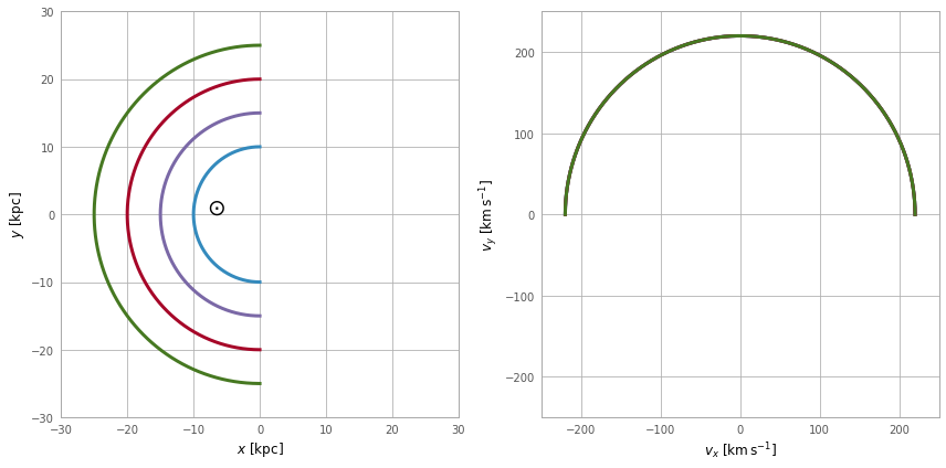
The transformations also work in the opposite direction. This can be useful for transforming simulated or theoretical data to observable quantities. As an example, we’ll generate 4 theoretical circular orbits at different Galactocentric radii with the same circular velocity, and transform them to Heliocentric coordinates:

ring_distances = np.arange(10, 25+1, 5) * u.kpc
circ_velocity = 220 * u.km/u.s

phi_grid = np.linspace(90, 270, 512) * u.degree # grid of azimuths
ring_rep = coord.CylindricalRepresentation(
    rho=ring_distances[:,np.newaxis],
    phi=phi_grid[np.newaxis],
    z=np.zeros_like(ring_distances)[:,np.newaxis])

angular_velocity = (-circ_velocity / ring_distances).to(u.mas/u.yr,
                                                        u.dimensionless_angles())
ring_dif = coord.CylindricalDifferential(
    d_rho=np.zeros(phi_grid.shape)[np.newaxis]*u.km/u.s,
    d_phi=angular_velocity[:,np.newaxis],
    d_z=np.zeros(phi_grid.shape)[np.newaxis]*u.km/u.s
)

ring_rep = ring_rep.with_differentials(ring_dif)
gc_rings = coord.Galactocentric(ring_rep)

First, let’s visualize the geometry in Galactocentric coordinates. Here are the positions and velocities of the rings; note that in the velocity plot, the velocities of the 4 rings are identical and thus overlaid under the same curve:

fig,axes = plt.subplots(1, 2, figsize=(12,6))

# Positions
axes[0].plot(gc_rings.x.T, gc_rings.y.T, marker='None', linewidth=3)
axes[0].text(-8., 0, r'$\odot$', fontsize=20)

axes[0].set_xlim(-30, 30)
axes[0].set_ylim(-30, 30)

axes[0].set_xlabel('$x$ [kpc]')
axes[0].set_ylabel('$y$ [kpc]')

# Velocities
axes[1].plot(gc_rings.v_x.T, gc_rings.v_y.T, marker='None', linewidth=3)

axes[1].set_xlim(-250, 250)
axes[1].set_ylim(-250, 250)

axes[1].set_xlabel('$v_x$ [{0}]'.format((u.km/u.s).to_string("latex_inline")))
axes[1].set_ylabel('$v_y$ [{0}]'.format((u.km/u.s).to_string("latex_inline")))

fig.tight_layout()

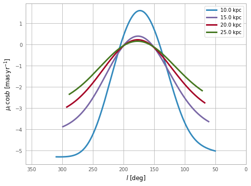
Now we can transform to Galactic coordinates and visualize the rings in observable coordinates:

gal_rings = gc_rings.transform_to(coord.Galactic)

fig,ax = plt.subplots(1, 1, figsize=(8,6))
for i in range(len(ring_distances)):
    ax.plot(gal_rings[i].l.degree, gal_rings[i].pm_l_cosb.value,
            label=str(ring_distances[i]), marker='None', linewidth=3)

ax.set_xlim(360, 0)

ax.set_xlabel('$l$ [deg]')
ax.set_ylabel(r'$\mu_l \, \cos b$ [{0}]'.format((u.mas/u.yr).to_string('latex_inline')))

ax.legend()

<matplotlib.legend.Legend at 0x1cc9f50a1c8>