Astropy examples
The group python4astronomers has some example files ready to download. You can Astropoy to do this.
[ ]:
from astropy.extern.six.moves.urllib import request
import tarfile
url = 'http://python4astronomers.github.io/_downloads/astropy_examples.tar'
tarfile.open(fileobj=request.urlopen(url), mode='r|').extractall()
# WARNING: AstropyDeprecationWarning: astropy.extern.six will be removed in 4.0, use the six module directly if it is still needed [astropy.extern.six]
[12]:
#cd "C:\Users\Kurt\Documents\Notebooks\astropy examples\"
[30]:
import numpy as np
import matplotlib.pyplot as plt
from astropy.io import fits
hdulist = fits.open(r'C:\Users\Kurt\Documents\Notebooks\astropy examples\data\gll_iem_v02_P6_V11_DIFFUSE.fit')
[6]:
hdulist.info()
Filename: C:\Users\Kurt\Documents\Notebooks\astropy examples\data\gll_iem_v02_P6_V11_DIFFUSE.fit
No.    Name      Ver    Type      Cards   Dimensions   Format
  0  PRIMARY       1 PrimaryHDU      34   (720, 360, 30)   float32
  1  ENERGIES      1 BinTableHDU     19   30R x 1C   [D]
[31]:
hdu = hdulist[0]
The hdu object then has two important attributes: data, which behaves like a Numpy array, can be used to access the data, and header, which behaves like a dictionary, can be used to access the header information. First, we can take a look at the data:
[8]:
hdu.data.shape
[8]:
(30, 360, 720)
This tells us that it is a 3-d cube. We can now take a peak at the header
[9]:
hdu.header
[9]:
SIMPLE  =                    T / Written by IDL:  Thu Jan 20 07:19:05 2011
BITPIX  =                  -32 /
NAXIS   =                    3 / number of data axes
NAXIS1  =                  720 / length of data axis 1
NAXIS2  =                  360 / length of data axis 2
NAXIS3  =                   30 / length of data axis 3
EXTEND  =                    T / FITS dataset may contain extensions
COMMENT   FITS (Flexible Image Transport System) format is defined in 'Astronomy
COMMENT   and Astrophysics', volume 376, page 359; bibcode: 2001A&A...376..359H
FLUX    =        8.42259635886 /
CRVAL1  =                   0. / Value of longitude in pixel CRPIX1
CDELT1  =                  0.5 / Step size in longitude
CRPIX1  =                360.5 / Pixel that has value CRVAL1
CTYPE1  = 'GLON-CAR'           / The type of parameter 1 (Galactic longitude in
CUNIT1  = 'deg     '           / The unit of parameter 1
CRVAL2  =                   0. / Value of latitude in pixel CRPIX2
CDELT2  =                  0.5 / Step size in latitude
CRPIX2  =                180.5 / Pixel that has value CRVAL2
CTYPE2  = 'GLAT-CAR'           / The type of parameter 2 (Galactic latitude in C
CUNIT2  = 'deg     '           / The unit of parameter 2
CRVAL3  =                  50. / Energy of pixel CRPIX3
CDELT3  =    0.113828620540137 / log10 of step size in energy (if it is logarith
CRPIX3  =                   1. / Pixel that has value CRVAL3
CTYPE3  = 'photon energy'      / Axis 3 is the spectra
CUNIT3  = 'MeV     '           / The unit of axis 3
CHECKSUM= '3fdO3caL3caL3caL'   / HDU checksum updated 2009-07-07T22:31:18
DATASUM = '2184619035'         / data unit checksum updated 2009-07-07T22:31:18
DATE    = '2009-07-07'         /
FILENAME= '$TEMPDIR/diffuse/gll_iem_v02.fit' /File name with version number
TELESCOP= 'GLAST   '           /
INSTRUME= 'LAT     '           /
ORIGIN  = 'LISOC   '           /LAT team product delivered from the LISOC
OBSERVER= 'MICHELSON'          /Instrument PI
HISTORY Scaled version of gll_iem_v02.fit for use with P6_V11_DIFFUSE
which shows that this is a Plate Carrée (-CAR) projection in Galactic Coordinates, and the third axis is photon energy. We can access individual header keywords using standard item notation:
[10]:
hdu.header['TELESCOP'] #'GLAST'
[10]:
'GLAST'
[11]:
hdu.header['INSTRUME'] #'LAT'
[11]:
'LAT'
we can plot one of the slices in photon energy:
[32]:
import matplotlib.pyplot as plt
fig = plt.figure()  # figsize(10,10)
plt.imshow(hdu.data[0,:,:], origin='lower')
fig.set_figheight(12)
fig.set_figwidth(15)
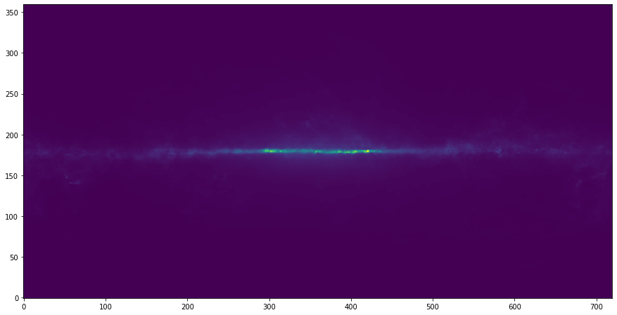
Note that this is just a plot of an array, so the coordinates are just pixel coordinates at this stage. The data is stored with longitude increasing to the right (the opposite of the normal convention), but the Level 3 problem at the bottom of this page shows how to correctly flip the image.
Modifying data or header information in a FITS file object is easy. We can update existing header keywords:
[ ]:
hdu.header['TELESCOP'] = "Fermi Gamma-ray Space Telescope"
[ ]:
hdu.header['MODIFIED'] = '26 Feb 2013' # adds a new keyword
and we can also change the data, for example extracting only the first slice in photon energy:
[ ]:
hdu.data = hdu.data[0,:,:]
Note that this does not change the original FITS file, simply the FITS file object in memory. Note that since the data is now 2-dimensional, we can remove the WCS keywords for the third dimension:
[ ]:
hdu.header.remove('CRPIX3')
hdu.header.remove('CRVAL3')
hdu.header.remove('CDELT3')
hdu.header.remove('CUNIT3')
hdu.header.remove('CTYPE3')
You can write the FITS file object to a file with:
[ ]:
hdu.writeto('lat_background_model_slice.fits')
if you want to simply write out this HDU to a file, or:
[ ]:
hdulist.writeto('lat_background_model_slice_allhdus.fits')
if you want to write out all of the original HDUs, including the modified one, to a file.
https://python4astronomers.github.io/astropy/fits.html
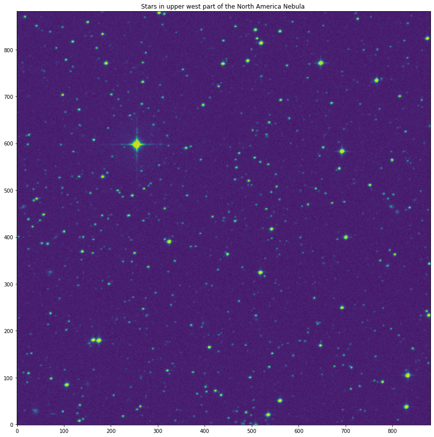
FITS file for skydata of object NGC 7000 (North America Nebula)
[2]:
import numpy as np
import matplotlib.pyplot as plt
from astropy.io import fits
hdulist = fits.open(r'C:\Users\Kurt\Documents\Notebooks\astropy examples\data\dss_search7000.fits')
[2]:
hdulist.info()
Filename: C:\Users\Kurt\Documents\Notebooks\astropy examples\data\dss_search7000.fits
No.    Name      Ver    Type      Cards   Dimensions   Format
  0  PRIMARY       1 PrimaryHDU     161   (882, 882)   int16
  1  xs.mask       1 TableHDU        25   1600R x 4C   [F6.2, F6.2, F6.2, F6.2]
[5]:
hdu = hdulist[0]
[4]:
hdu.data.shape
[4]:
(882, 882)
[5]:
hdu.header
[5]:
SIMPLE  =                    T /FITS: Compliance
BITPIX  =                   16 /FITS: I*2 Data
NAXIS   =                    2 /FITS: 2-D Image Data
NAXIS1  =                  882 /FITS: X Dimension
NAXIS2  =                  882 /FITS: Y Dimension
EXTEND  =                    T /FITS: File can contain extensions
DATE    = '2019-11-17        '  /FITS: Creation Date
ORIGIN  = 'STScI/MAST'         /GSSS: STScI Digitized Sky Survey
SURVEY  = 'AAO-SES '           /GSSS: Sky Survey
REGION  = 'XS447   '           /GSSS: Region Name
PLATEID = 'A04V    '           /GSSS: Plate ID
SCANNUM = '01      '           /GSSS: Scan Number
DSCNDNUM= '00      '           /GSSS: Descendant Number
TELESCID=                    4 /GSSS: Telescope ID
BANDPASS=                   35 /GSSS: Bandpass Code
COPYRGHT= 'AAO/ROE '           /GSSS: Copyright Holder
SITELAT =              -31.277 /Observatory: Latitude
SITELONG=              210.934 /Observatory: Longitude
TELESCOP= 'UK Schmidt - Doubl' /Observatory: Telescope
INSTRUME= 'Photographic Plate' /Detector: Photographic Plate
EMULSION= 'IIIaF   '           /Detector: Emulsion
FILTER  = 'RG610   '           /Detector: Filter
PLTSCALE=                67.20 /Detector: Plate Scale arcsec per mm
PLTSIZEX=              355.000 /Detector: Plate X Dimension mm
PLTSIZEY=              355.000 /Detector: Plate Y Dimension mm
PLATERA =        219.202580000 /Observation: Field centre RA degrees
PLATEDEC=       -30.2292770000 /Observation: Field centre Dec degrees
PLTLABEL= 'OR14304 '           /Observation: Plate Label
DATE-OBS= '1991-04-13T15:46:00' /Observation: Date/Time
EXPOSURE=                 60.0 /Observation: Exposure Minutes
PLTGRADE= 'A3      '           /Observation: Plate Grade
OBSHA   =             0.500000 /Observation: Hour Angle
OBSZD   =              6.57670 /Observation: Zenith Distance
AIRMASS =              1.00661 /Observation: Airmass
REFBETA =        66.3196420000 /Observation: Refraction Coeff
REFBETAP=     -0.0820000000000 /Observation: Refraction Coeff
REFK1   =        21255.1180000 /Observation: Refraction Coeff
REFK2   =       -4467.87440000 /Observation: Refraction Coeff
CNPIX1  =                11347 /Scan: X Corner
CNPIX2  =                12051 /Scan: Y Corner
XPIXELS =                23040 /Scan: X Dimension
YPIXELS =                23040 /Scan: Y Dimension
XPIXELSZ=              15.1872 /Scan: Pixel Size microns
YPIXELSZ=              15.1872 /Scan: Pixel Size microns
PPO1    =       -3069417.00000 /Scan: Orientation Coeff
PPO2    =       0.000000000000 /Scan: Orientation Coeff
PPO3    =        177500.000000 /Scan: Orientation Coeff
PPO4    =       0.000000000000 /Scan: Orientation Coeff
PPO5    =        3069417.00000 /Scan: Orientation Coeff
PPO6    =        177500.000000 /Scan: Orientation Coeff
PLTRAH  =                   14 /Astrometry: Plate Centre H
PLTRAM  =                   36 /Astrometry: Plate Centre M
PLTRAS  =                58.09 /Astrometry: Plate Centre S
PLTDECSN= '-       '           /Astrometry: Plate Centre +/-
PLTDECD =                   30 /Astrometry: Plate Centre D
PLTDECM =                   13 /Astrometry: Plate Centre M
PLTDECS =                  0.4 /Astrometry: Plate Centre S
EQUINOX =               2000.0 /Astrometry: Equinox
AMDX1   =        67.1500087237 /Astrometry: GSC1 Coeff
AMDX2   =      -0.102575695834 /Astrometry: GSC1 Coeff
AMDX3   =       -293.778893318 /Astrometry: GSC1 Coeff
AMDX4   =  -3.33870873108E-005 /Astrometry: GSC1 Coeff
AMDX5   =   6.38394957927E-006 /Astrometry: GSC1 Coeff
AMDX6   =  -1.05213797334E-005 /Astrometry: GSC1 Coeff
AMDX7   =       0.000000000000 /Astrometry: GSC1 Coeff
AMDX8   =   2.42449438155E-006 /Astrometry: GSC1 Coeff
AMDX9   =  -7.13218045949E-008 /Astrometry: GSC1 Coeff
AMDX10  =   2.45363445160E-006 /Astrometry: GSC1 Coeff
AMDX11  =  -4.75351668260E-008 /Astrometry: GSC1 Coeff
AMDX12  =       0.000000000000 /Astrometry: GSC1 Coeff
AMDX13  =       0.000000000000 /Astrometry: GSC1 Coeff
AMDX14  =       0.000000000000 /Astrometry: GSC1 Coeff
AMDX15  =       0.000000000000 /Astrometry: GSC1 Coeff
AMDX16  =       0.000000000000 /Astrometry: GSC1 Coeff
AMDX17  =       0.000000000000 /Astrometry: GSC1 Coeff
AMDX18  =       0.000000000000 /Astrometry: GSC1 Coeff
AMDX19  =       0.000000000000 /Astrometry: GSC1 Coeff
AMDX20  =       0.000000000000 /Astrometry: GSC1 Coeff
AMDY1   =        67.1462956300 /Astrometry: GSC1 Coeff
AMDY2   =       0.111494176722 /Astrometry: GSC1 Coeff
AMDY3   =        125.530051071 /Astrometry: GSC1 Coeff
AMDY4   =   1.09223680595E-005 /Astrometry: GSC1 Coeff
AMDY5   =  -2.02805190630E-005 /Astrometry: GSC1 Coeff
AMDY6   =   1.07085463778E-005 /Astrometry: GSC1 Coeff
AMDY7   =       0.000000000000 /Astrometry: GSC1 Coeff
AMDY8   =   2.45598733465E-006 /Astrometry: GSC1 Coeff
AMDY9   =   8.05323459363E-009 /Astrometry: GSC1 Coeff
AMDY10  =   2.48318049954E-006 /Astrometry: GSC1 Coeff
AMDY11  =   4.90083901307E-009 /Astrometry: GSC1 Coeff
AMDY12  =       0.000000000000 /Astrometry: GSC1 Coeff
AMDY13  =       0.000000000000 /Astrometry: GSC1 Coeff
AMDY14  =       0.000000000000 /Astrometry: GSC1 Coeff
AMDY15  =       0.000000000000 /Astrometry: GSC1 Coeff
AMDY16  =       0.000000000000 /Astrometry: GSC1 Coeff
AMDY17  =       0.000000000000 /Astrometry: GSC1 Coeff
AMDY18  =       0.000000000000 /Astrometry: GSC1 Coeff
AMDY19  =       0.000000000000 /Astrometry: GSC1 Coeff
AMDY20  =       0.000000000000 /Astrometry: GSC1 Coeff
AMDREX1 =        67.1512980022 /Astrometry: GSC2 Coeff
AMDREX2 =      -0.103702972347 /Astrometry: GSC2 Coeff
AMDREX3 =       -293.773745123 /Astrometry: GSC2 Coeff
AMDREX4 =  -1.85785729331E-006 /Astrometry: GSC2 Coeff
AMDREX5 =  -2.49637342475E-006 /Astrometry: GSC2 Coeff
AMDREX6 =   5.90460785575E-007 /Astrometry: GSC2 Coeff
AMDREX7 =       0.000000000000 /Astrometry: GSC2 Coeff
AMDREX8 =       0.000000000000 /Astrometry: GSC2 Coeff
AMDREX9 =       0.000000000000 /Astrometry: GSC2 Coeff
AMDREX10=       0.000000000000 /Astrometry: GSC2 Coeff
AMDREX11=       0.000000000000 /Astrometry: GSC2 Coeff
AMDREX12=       0.000000000000 /Astrometry: GSC2 Coeff
AMDREX13=       0.000000000000 /Astrometry: GSC2 Coeff
AMDREX14=       0.000000000000 /Astrometry: GSC2 Coeff
AMDREX15=       0.000000000000 /Astrometry: GSC2 Coeff
AMDREX16=       0.000000000000 /Astrometry: GSC2 Coeff
AMDREX17=       0.000000000000 /Astrometry: GSC2 Coeff
AMDREX18=       0.000000000000 /Astrometry: GSC2 Coeff
AMDREX19=       0.000000000000 /Astrometry: GSC2 Coeff
AMDREX20=       0.000000000000 /Astrometry: GSC2 Coeff
AMDREY1 =        67.1487327610 /Astrometry: GSC2 Coeff
AMDREY2 =       0.111633779049 /Astrometry: GSC2 Coeff
AMDREY3 =        125.565175070 /Astrometry: GSC2 Coeff
AMDREY4 =  -3.77188918418E-006 /Astrometry: GSC2 Coeff
AMDREY5 =  -4.94510410020E-007 /Astrometry: GSC2 Coeff
AMDREY6 =   4.27863272953E-006 /Astrometry: GSC2 Coeff
AMDREY7 =       0.000000000000 /Astrometry: GSC2 Coeff
AMDREY8 =       0.000000000000 /Astrometry: GSC2 Coeff
AMDREY9 =       0.000000000000 /Astrometry: GSC2 Coeff
AMDREY10=       0.000000000000 /Astrometry: GSC2 Coeff
AMDREY11=       0.000000000000 /Astrometry: GSC2 Coeff
AMDREY12=       0.000000000000 /Astrometry: GSC2 Coeff
AMDREY13=       0.000000000000 /Astrometry: GSC2 Coeff
AMDREY14=       0.000000000000 /Astrometry: GSC2 Coeff
AMDREY15=       0.000000000000 /Astrometry: GSC2 Coeff
AMDREY16=       0.000000000000 /Astrometry: GSC2 Coeff
AMDREY17=       0.000000000000 /Astrometry: GSC2 Coeff
AMDREY18=       0.000000000000 /Astrometry: GSC2 Coeff
AMDREY19=       0.000000000000 /Astrometry: GSC2 Coeff
AMDREY20=       0.000000000000 /Astrometry: GSC2 Coeff
ASTRMASK= 'xs.mask '           /Astrometry: GSC2 Mask
WCSAXES =                    2 /GetImage: Number WCS axes
WCSNAME = 'DSS               ' /GetImage: Local WCS approximation from full plat
RADESYS = 'ICRS              ' /GetImage: GSC-II calibration using ICRS system
CTYPE1  = 'RA---TAN          ' /GetImage: RA-Gnomic projection
CRPIX1  =           441.500000 /GetImage: X reference pixel
CRVAL1  =           219.114583 /GetImage: RA of reference pixel
CUNIT1  = 'deg               ' /GetImage: degrees
CTYPE2  = 'DEC--TAN          ' /GetImage: Dec-Gnomic projection
CRPIX2  =           441.500000 /GetImage: Y reference pixel
CRVAL2  =           -29.953980 /GetImage: Dec of reference pixel
CUNIT2  = 'deg               ' /Getimage: degrees
CD1_1   =        -0.0002832882 /GetImage: rotation matrix coefficient
CD1_2   =        -0.0000001545 /GetImage: rotation matrix coefficient
CD2_1   =        -0.0000001224 /GetImage: rotation matrix coefficient
CD2_2   =         0.0002832770 /GetImage: rotation matrix coefficient
OBJECT  = 'data              ' /GetImage: Requested Object Name
DATAMIN =                10990 /GetImage: Minimum returned pixel value
DATAMAX =                29619 /GetImage: Maximum returned pixel value
OBJCTRA = '14 36 27.490      ' /GetImage: Requested Right Ascension (J2000)
OBJCTDEC= '-29 57 14.20      ' /GetImage: Requested Declination (J2000)
OBJCTX  =             11788.14 /GetImage: Requested X on plate (pixels)
OBJCTY  =             12492.19 /GetImage: Requested Y on plate (pixels)
[27]:
import matplotlib.pyplot as plt
fig = plt.figure()  # figsize(10,10)
ax= plt.axes()
plt.imshow(hdu.data, origin='lower')  # hdu.data[0,:]
fig.set_figheight(15)
fig.set_figwidth(15)
plt.title("Stars in upper west part of the North America Nebula ")
[27]:
Text(0.5, 1.0, 'Stars in upper west part of the North America Nebula ')
[26]:
from IPython.display import Image
imshow=Image(url="https://lh5.googleusercontent.com/YrxwnafAGfyAV30hWVIJP74plnbewicbYTbO89cbqprJge2gpdsnOrle9yWJUuqCHGXIrOltOh9nN0SRwdDeVa012wMVHfejYK7GwlcJOHx8q1kam4NR12hEGosq4reBcXuIv0nI")
imshow
[26]:

[ ]: