Runoff hydrographs of Ahr tributaries

Author: Van Oproy Kurt

The objectif is to make a realistic hydrograph for the destroyed measurestation at Altenahr, based on the Ahr's tributaries.
Therefore, the watersheds of the important tributaries of the Ahr were delineated seperately, selecting only the tributaries of the Ahr upstream from Altenahr. For each watersheds a runoff calculation was performed, and the discharge values were transposed to an Excel file.
The first combined results gave a reaction profile for the discharge at Altenahr that started 1.5 hours earlier than the observed flow.

  • Was this delay the result of the series of debris-clogged bridges, that held the water mass up?
    • how many bridges are there between Müsch and Altenahr?
      • 72 bridges have been severely damaged or destroyed in the whole Ahr valley (source: German army officer)
    • for a debit of 300 m³/s, how long does it take to overcome a 50 cm, or a 2 meter, bridge height over a 30 to 60 meter width?
  • Later in this work we'll show the phenomenon of hysteresis for the flood wave debit-water level curve.
    • The peak of the debit happens some time before that of the water level.
Out[2]:
3.1416
Reading sheet Blad2

The measure stations of the Ahr

  • Parameters Maximum_Abfluss_m³s, Maximum_Wasserstand and HQ 100 (m³/s) are based on the recordings of the gauging stations before the 2021 deluge.
  • Parameter HW_waterlevel is based on factual data of the 2021 deluge, in some cases based on highwater marks with eyewitness testimony.
    • The evaluation of the water height was done by comparing water bed and highwater mark height with online German elevation maps.
  • Parameter HW_Debit is derived from the 'model' which calculates a debit from water levels.
  • The recorded time for the sensors is normally without summertime correction. However, I did not apply this kind of correction, because:
    • I cannot know if a more recently installed sensor has automatic summertime/wintertime correction onboard, nor if this function had been enabled.
    • This omission might explain a big part of the lag visible in the calculated vs. recorded outflows, but I did not want to create confusion.

Official version

Out[5]:
Kirmutscheid Niederadenau Kreuzberg Altenahr Müsch Denn
Pegelname
Gewässer Trierbach Adenauerbach Sahrbach Ahr Ahr Kesselingerbach
Messstellennummer 2718050500 2718085500 2718090200 2718040300 2718010800 2718070900
Stromgebiet Ahr+-+Rhein Ahr+-+Rhein Ahr+-+Rhein Rhein Rhein Ahr+-+Rhein
Einzugsgebiet (km2) 88.0 57.03 45.0 746.0 352.65 94.0
Lage oberhalb Mündung (km) 3.5 1.26 1 31.7 63 0.7
Pegelnullpunkt 317.75 222.01 178.89 160.52 292.77 191.15
Eingerichtet 1945-01-01 00:00:00 2013-11-13 00:00:00 1956-01-01 00:00:00 1991-01-01 00:00:00 1952-01-01 00:00:00 1955-01-01 00:00:00
Lat 50.37 50.44 50.51 50.52 50.39 50.48
Long 6.84 6.93 6.97 6.99 6.83 6.98
Maximum_Abfluss_m³s 82.3 NaN 17.9 236.0 132.0 71.6
Maximum_Wasserstand 269.0 NaN 199.0 371.0 273.0 241.0
HQ 100 (m³/s) 94.7 NaN 18.9 241.0 152.0 67.8
HW_waterlevel 307.0 204.0 327.0 575.0 304.25 293.0
HW_Debit 104.13 69.66 66.44 332.27 320.0 97.38
Outage_time NaT NaT 2021-07-14 18:30:00 2021-07-14 19:15:00 NaT NaT
Exceedance 0.1 NaN 2.52 0.38 1.11 0.44

Some facts about the flood, with references, collected from the media:

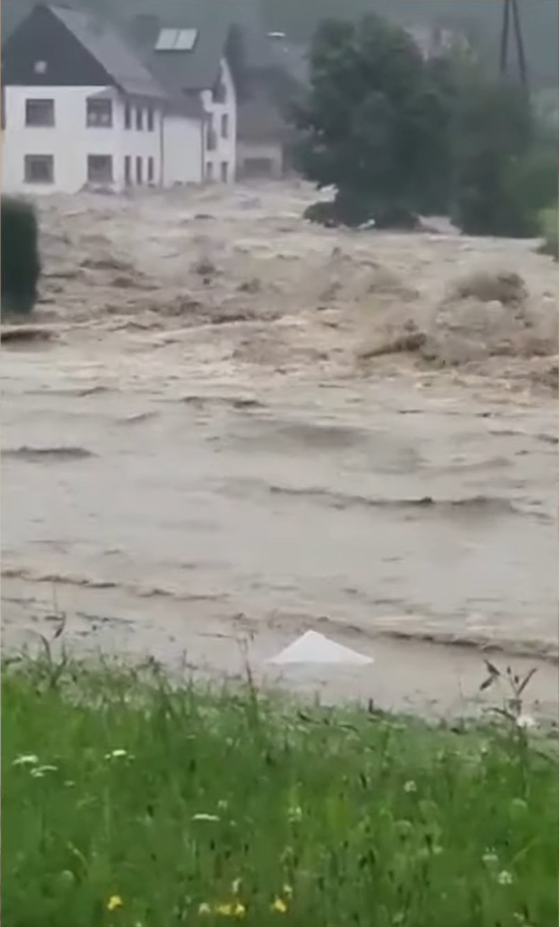
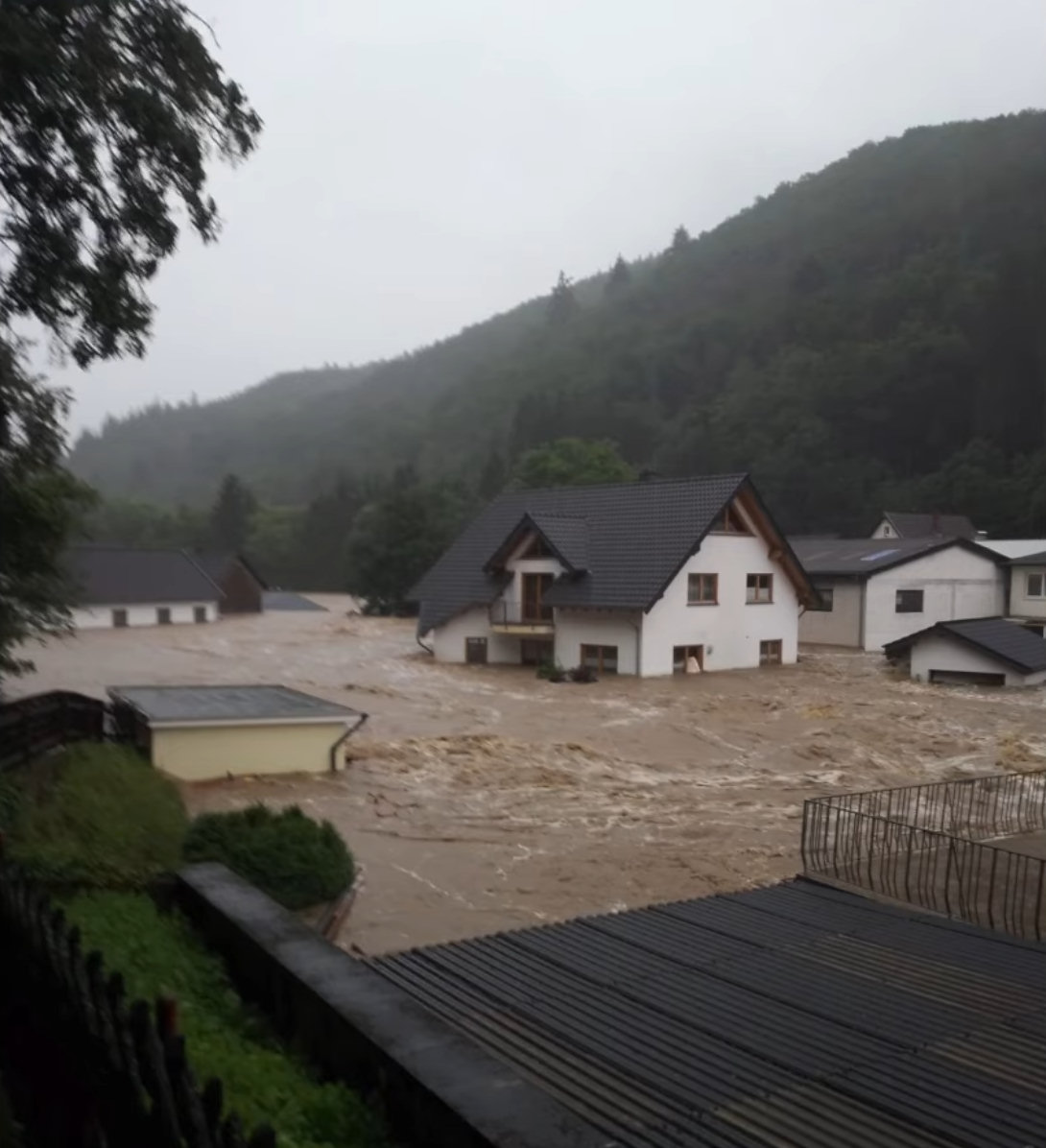
Video of houses of the Uberdorfstrasse 2 and 4 in Insul, where the height of floodwave - shown in the video - was at least 1.5 - 2 meters above the street level.

  • Arh level : 217.5, water level +- 2.75- 3 meter.
  • Insul is 17 km stream downward from Müsch. Time to travel is 1.5 hours, or less in case of a flood...
  • The surface area for the water to pass there is 100-110 m², considering the buildings that kept standing after the flood.
  • I you watch closely, you notice that the flood doesn't follow the river, as the river level is still lower than the bypassing flood.

Video interview with local Christof Pätz in Altenburg:

  • The peak water level was visible on his house at 6-6.5 m height, which was reached on 14-07 22:30, "9 meters from the waterbed".
  • His house is 155 meters away from the Ahr, at 168 masl.
  • This location is 1.1 km upstream from the Altenahr station.

Factual version

I added my own collected information, starting from feature/row "HQ 100 (m³/s)".

Out[9]:
Kirmutscheid Niederadenau Kreuzberg Altenahr Müsch Denn
Pegelname
Gewässer Trierbach Adenauerbach Sahrbach Ahr Ahr Kesselingerbach
Messstellennummer 2718050500 2718085500 2718090200 2718040300 2718010800 2718070900
Stromgebiet Ahr+-+Rhein Ahr+-+Rhein Ahr+-+Rhein Rhein Rhein Ahr+-+Rhein
Einzugsgebiet (km2) 88.0 57.03 45.0 746.0 352.65 94.0
Lage oberhalb Mündung (km) 3.5 1.26 1 31.7 63 0.7
Pegelnullpunkt 317.75 222.01 178.89 160.52 292.77 191.15
Eingerichtet 1945-01-01 00:00:00 2013-11-13 00:00:00 1956-01-01 00:00:00 1991-01-01 00:00:00 1952-01-01 00:00:00 1955-01-01 00:00:00
Lat 50.37 50.44 50.51 50.52 50.39 50.48
Long 6.84 6.93 6.97 6.99 6.83 6.98
Maximum_Abfluss_m³s 82.3 NaN 17.9 236.0 132.0 71.6
Maximum_Wasserstand 269.0 NaN 199.0 371.0 273.0 241.0
HQ 100 (m³/s) 94.7 NaN 18.9 241.0 152.0 67.8
HW_waterlevel 307.0 204.0 550.0 975.0 400.0 293.0
HW_Debit 104.13 69.66 115.0 850.0 320.0 97.38
Outage_time NaT NaT 2021-07-14 18:30:00 2021-07-14 19:15:00 NaT NaT
Exceedance 0.1 NaN 5.08 2.53 1.11 0.44
Out[3]:
Flow rate (m³/s)
Time
2021-07-12 00:00:00 0.00e+00
2021-07-12 00:15:00 0.00e+00
2021-07-12 00:30:00 0.00e+00
2021-07-12 00:45:00 0.00e+00
2021-07-12 01:00:00 0.00e+00
... ...
2021-07-17 03:15:00 4.42e-06
2021-07-17 03:30:00 0.00e+00
2021-07-17 03:45:00 0.00e+00
2021-07-17 04:00:00 0.00e+00
2021-07-17 04:15:00 0.00e+00

498 rows × 1 columns

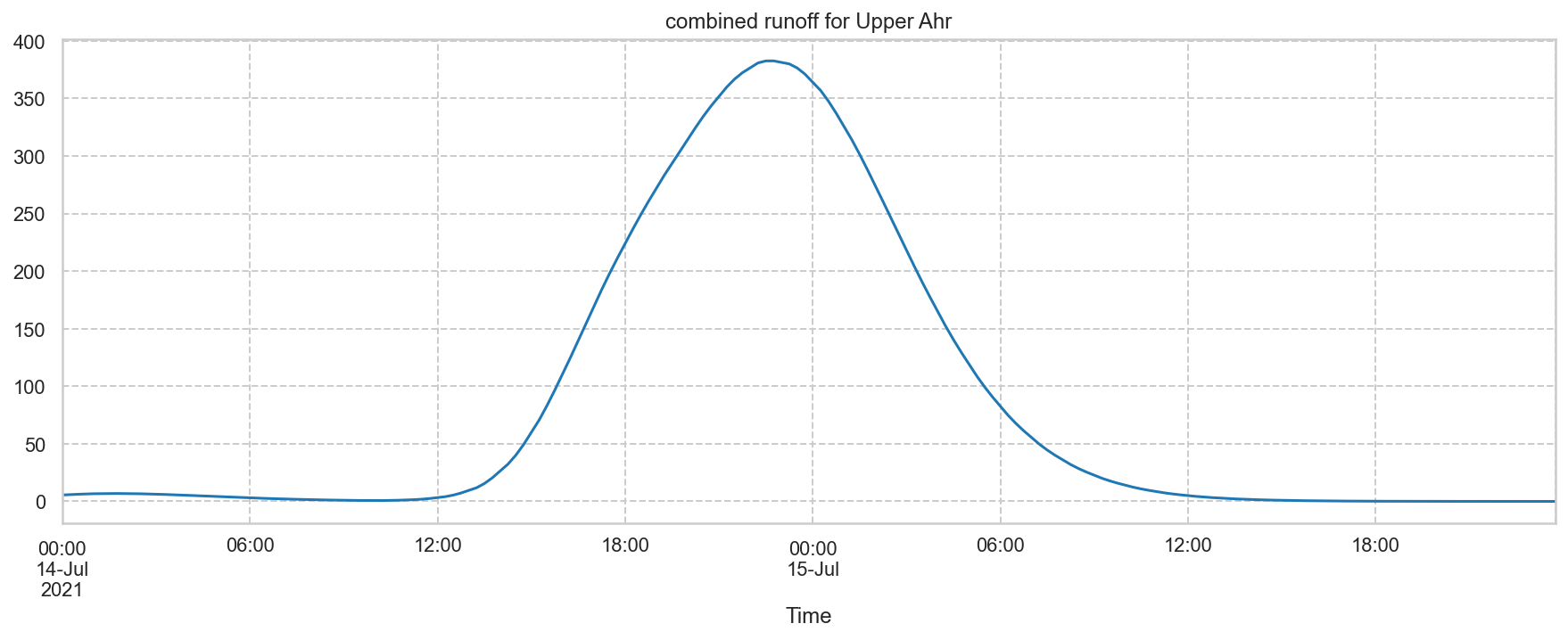
The plot 'MidAhr(Fr)' contains the aggregated flowrate, which is based on the precipitation of the nearest location with pluvio data I could find, for places like Freilingen, Barweiler, ...

Out[6]:
Flow rate (m³/s) Freilingen rain
Time
2021-06-10 00:00:00 0.0 NaN
2021-06-10 01:00:00 0.0 NaN
2021-06-10 02:00:00 0.0 NaN
2021-06-10 03:00:00 0.0 NaN
2021-06-10 04:00:00 0.0 NaN
... ... ...
2021-07-21 12:00:00 0.0 NaN
2021-07-21 13:00:00 0.0 NaN
2021-07-21 14:00:00 0.0 NaN
2021-07-21 15:00:00 0.0 NaN
2021-07-21 16:00:00 0.0 NaN

1001 rows × 2 columns

Several surface runoff hydrographs

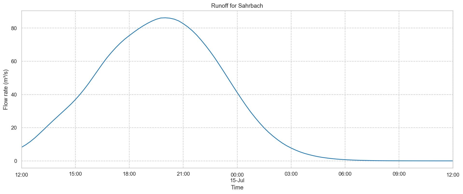
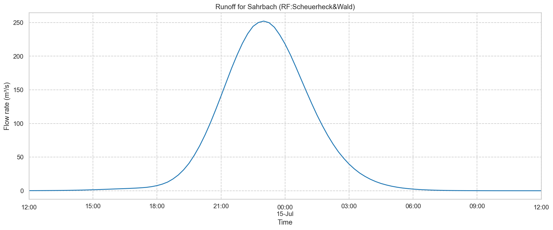
The first set is representing the Sahrbach catchment surface runoff.

The runoff values were calculated for these tributaries:

['Sahr', 'Liers', 'Armuths', 'Ans', 'Nohner', 'Trier', 'Wirft', 'Adenauer', 'Denn', 'Staffel', 'Vischel', 'UpperAhr']
Out[9]:
Flow rate (m³/s)
Time
2021-07-07 00:00:00 0.0
2021-07-07 00:15:00 0.0
2021-07-07 00:30:00 0.0
2021-07-07 00:45:00 0.0
2021-07-07 01:00:00 0.0
... ...
2021-07-24 11:15:00 0.0
2021-07-24 11:30:00 0.0
2021-07-24 11:45:00 0.0
2021-07-24 12:00:00 0.0
2021-07-24 12:15:00 0.0

1682 rows × 1 columns

Sahrbach flood Kirchsahr Sahrbach flood Kirchsahr 2, source Feierwehr Kirchsahr
Sahrbach start of flood in Kirchsahr Sahrbach flood Kirchsahr 2

Rainfall data of Freilingen pluviometer

Rainfall data of Scheuerheck & Wald pluviometers

we merge the individual hydrographs.

Out[13]:
Flow rate (m³/s)Sahr Flow rate (m³/s)Liers Flow rate (m³/s) Flow rate (m³/s)Ans Flow rate (m³/s)Nohner Flow rate (m³/s)Trier Flow rate (m³/s)Wirft Flow rate (m³/s)Adenauer
Time
2021-07-13 00:00:00 0.00e+00 0.00e+00 0.00e+00 0.00e+00 0.00e+00 0.00e+00 0.00e+00 4.02
2021-07-13 01:00:00 0.00e+00 0.00e+00 0.00e+00 0.00e+00 0.00e+00 1.95e-06 6.04e-07 7.66
2021-07-13 02:00:00 0.00e+00 0.00e+00 0.00e+00 0.00e+00 0.00e+00 6.30e-04 1.71e-04 9.27
2021-07-13 03:00:00 2.29e-04 2.27e-07 1.28e-06 2.11e-07 0.00e+00 7.49e-03 1.74e-03 9.13
2021-07-13 04:00:00 2.32e-03 1.86e-04 3.31e-04 3.06e-04 0.00e+00 2.72e-02 5.40e-03 13.34
... ... ... ... ... ... ... ... ...
2021-07-15 12:00:00 2.30e-03 4.49e-03 1.52e-01 1.12e-05 9.17e-03 7.96e-04 NaN 0.00
2021-07-15 13:00:00 6.09e-04 1.48e-03 6.62e-02 0.00e+00 3.27e-03 0.00e+00 NaN 0.00
2021-07-15 14:00:00 0.00e+00 2.30e-04 2.80e-02 0.00e+00 1.20e-03 NaN NaN 0.00
2021-07-15 15:00:00 0.00e+00 4.74e-05 1.15e-02 0.00e+00 4.10e-04 NaN NaN 0.00
2021-07-15 16:00:00 0.00e+00 1.73e-05 3.91e-03 0.00e+00 1.56e-05 0.00e+00 0.00e+00 0.00

65 rows × 8 columns

Out[15]:
Flow rate (m³/s)Sahr Flow rate (m³/s)Liers Flow rate (m³/s) Flow rate (m³/s)Ans Flow rate (m³/s)Nohner Flow rate (m³/s)Trier Flow rate (m³/s)Wirft Flow rate (m³/s)Adenauer Flow rate (m³/s)Denn Flow rate (m³/s)Staffel Flow rate (m³/s)Vischel
Time
2021-07-13 00:00:00 0.00e+00 0.00e+00 0.00e+00 0.00e+00 0.00e+00 0.00e+00 0.00e+00 4.02 3.82 3.15 0.02
2021-07-13 01:00:00 0.00e+00 0.00e+00 0.00e+00 0.00e+00 0.00e+00 1.95e-06 6.04e-07 7.66 4.28 5.76 0.10
2021-07-13 02:00:00 0.00e+00 0.00e+00 0.00e+00 0.00e+00 0.00e+00 6.30e-04 1.71e-04 9.27 2.77 6.59 0.17
2021-07-13 03:00:00 2.29e-04 2.27e-07 1.28e-06 2.11e-07 0.00e+00 7.49e-03 1.74e-03 9.13 3.71 6.21 0.24
2021-07-13 04:00:00 2.32e-03 1.86e-04 3.31e-04 3.06e-04 0.00e+00 2.72e-02 5.40e-03 13.34 9.56 9.73 0.26
... ... ... ... ... ... ... ... ... ... ... ...
2021-07-15 12:00:00 2.30e-03 4.49e-03 1.52e-01 1.12e-05 9.17e-03 7.96e-04 NaN 0.00 0.00 0.00 0.00
2021-07-15 13:00:00 6.09e-04 1.48e-03 6.62e-02 0.00e+00 3.27e-03 0.00e+00 NaN 0.00 0.00 0.00 0.00
2021-07-15 14:00:00 0.00e+00 2.30e-04 2.80e-02 0.00e+00 1.20e-03 NaN NaN 0.00 0.00 0.00 0.00
2021-07-15 15:00:00 0.00e+00 4.74e-05 1.15e-02 0.00e+00 4.10e-04 NaN NaN 0.00 0.00 0.00 0.00
2021-07-15 16:00:00 0.00e+00 1.73e-05 3.91e-03 0.00e+00 1.56e-05 0.00e+00 0.00e+00 0.00 0.00 0.00 0.00

65 rows × 11 columns

Out[16]:
Flow rate (m³/s)
Time
2021-07-12 00:00:00 0.00e+00
2021-07-12 00:15:00 0.00e+00
2021-07-12 00:30:00 0.00e+00
2021-07-12 00:45:00 0.00e+00
2021-07-12 01:00:00 0.00e+00
... ...
2021-07-17 03:15:00 4.42e-06
2021-07-17 03:30:00 0.00e+00
2021-07-17 03:45:00 0.00e+00
2021-07-17 04:00:00 0.00e+00
2021-07-17 04:15:00 0.00e+00

498 rows × 1 columns

Out[17]:
Flow rate (m³/s)Sahr Flow rate (m³/s)Liers Flow rate (m³/s) Flow rate (m³/s)Ans Flow rate (m³/s)Nohner Flow rate (m³/s)Trier Flow rate (m³/s)Wirft Flow rate (m³/s)Adenauer Flow rate (m³/s)Denn Flow rate (m³/s)Staffel Flow rate (m³/s)Vischel Flow rate (m³/s)UpperAhr Flow rate (m³/s)Weiden
Time
2021-07-13 00:00:00 0.00e+00 0.00e+00 0.00e+00 0.00e+00 0.00e+00 0.00e+00 0.00e+00 4.02 3.82 3.15 0.02 0.00e+00 3.57
2021-07-13 01:00:00 0.00e+00 0.00e+00 0.00e+00 0.00e+00 0.00e+00 1.95e-06 6.04e-07 7.66 4.28 5.76 0.10 0.00e+00 6.04
2021-07-13 02:00:00 0.00e+00 0.00e+00 0.00e+00 0.00e+00 0.00e+00 6.30e-04 1.71e-04 9.27 2.77 6.59 0.17 0.00e+00 6.34
2021-07-13 03:00:00 2.29e-04 2.27e-07 1.28e-06 2.11e-07 0.00e+00 7.49e-03 1.74e-03 9.13 3.71 6.21 0.24 4.29e-07 5.85
2021-07-13 04:00:00 2.32e-03 1.86e-04 3.31e-04 3.06e-04 0.00e+00 2.72e-02 5.40e-03 13.34 9.56 9.73 0.26 2.00e-04 10.14
... ... ... ... ... ... ... ... ... ... ... ... ... ...
2021-07-15 12:00:00 2.30e-03 4.49e-03 1.52e-01 1.12e-05 9.17e-03 7.96e-04 NaN 0.00 0.00 0.00 0.00 1.04e+01 0.00
2021-07-15 13:00:00 6.09e-04 1.48e-03 6.62e-02 0.00e+00 3.27e-03 0.00e+00 NaN 0.00 0.00 0.00 0.00 6.15e+00 0.00
2021-07-15 14:00:00 0.00e+00 2.30e-04 2.80e-02 0.00e+00 1.20e-03 NaN NaN 0.00 0.00 0.00 0.00 3.59e+00 0.00
2021-07-15 15:00:00 0.00e+00 4.74e-05 1.15e-02 0.00e+00 4.10e-04 NaN NaN 0.00 0.00 0.00 0.00 2.06e+00 0.00
2021-07-15 16:00:00 0.00e+00 1.73e-05 3.91e-03 0.00e+00 1.56e-05 0.00e+00 0.00e+00 0.00 0.00 0.00 0.00 1.16e+00 0.00

65 rows × 13 columns

Out[18]:
Time
2021-07-13 00:00:00     3.57
2021-07-13 01:00:00     6.04
2021-07-13 02:00:00     6.34
2021-07-13 03:00:00     5.85
2021-07-13 04:00:00    10.14
                       ...  
2021-07-15 12:00:00     0.00
2021-07-15 13:00:00     0.00
2021-07-15 14:00:00     0.00
2021-07-15 15:00:00     0.00
2021-07-15 16:00:00     0.00
Name: Flow rate (m³/s)Weiden, Length: 65, dtype: float64

Summation of the discharges of the streams upstream of Altenahr

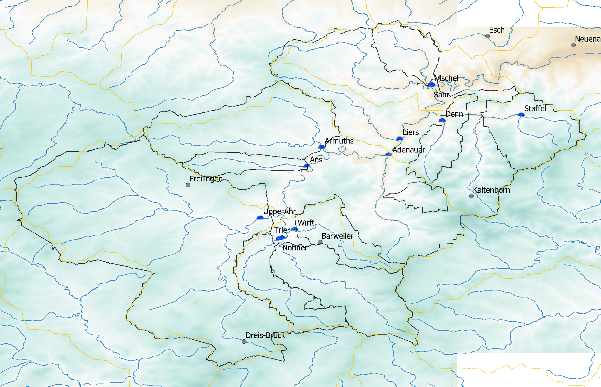
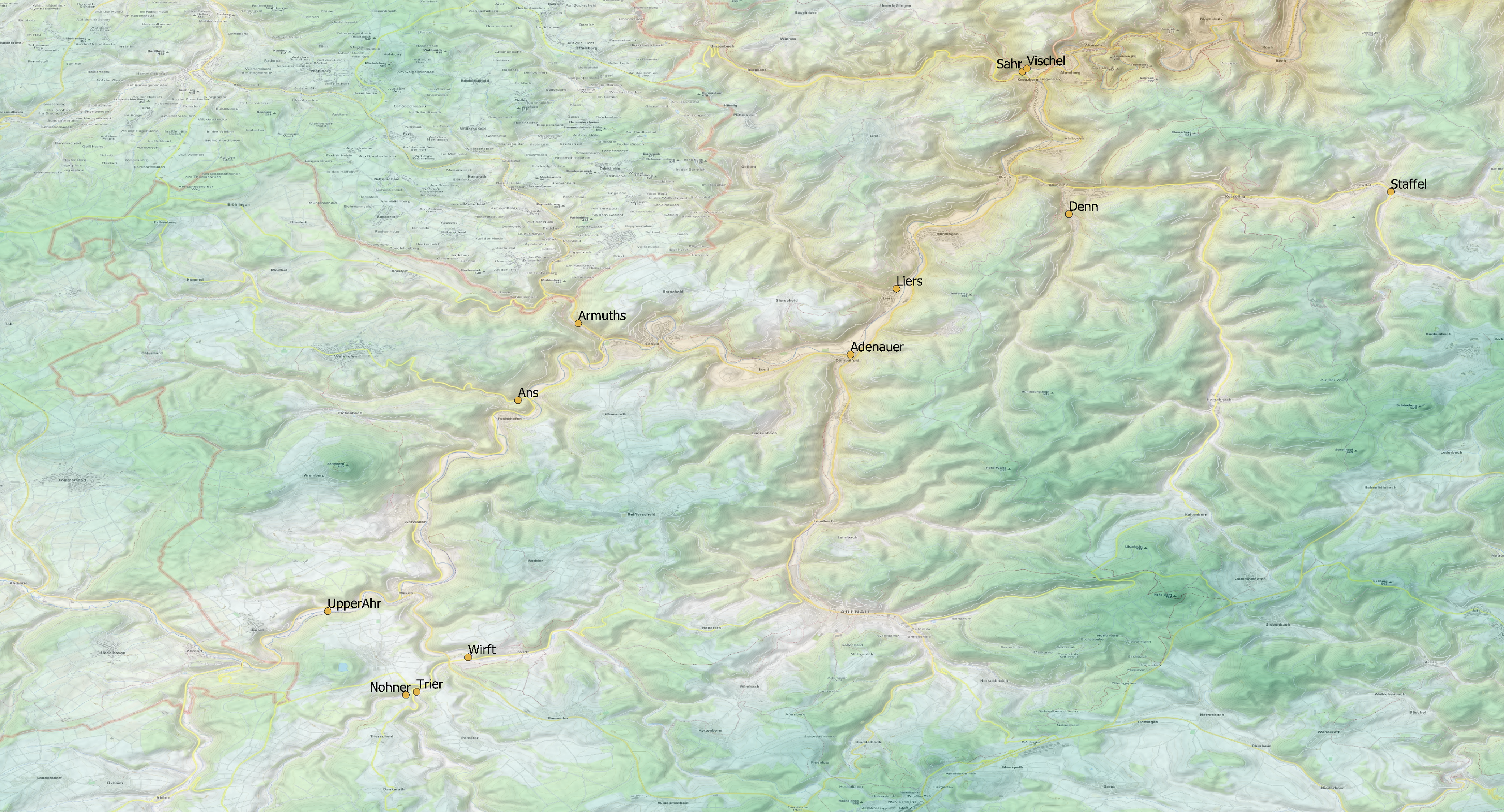
Streams and outlet points location

Land use proportions

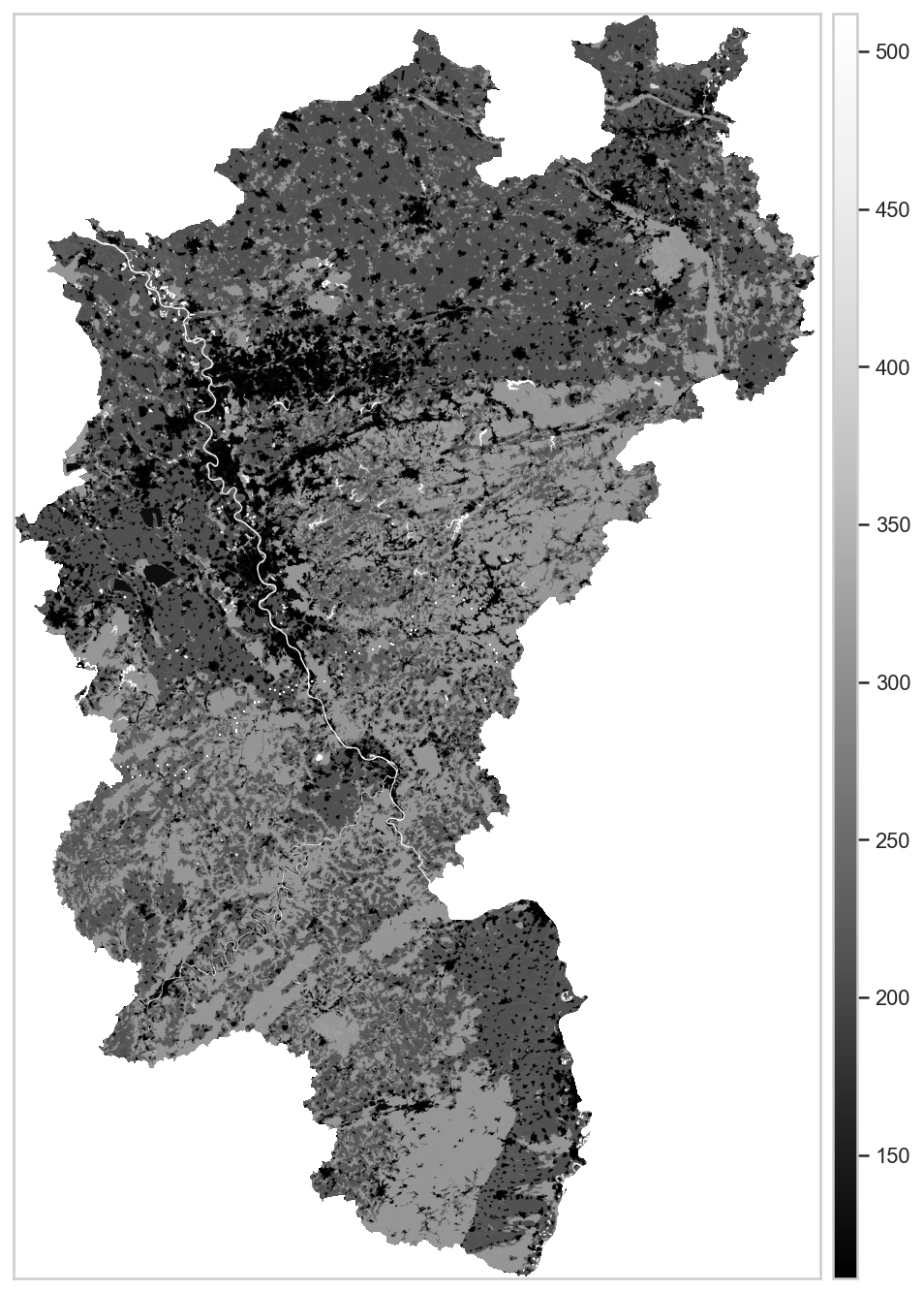
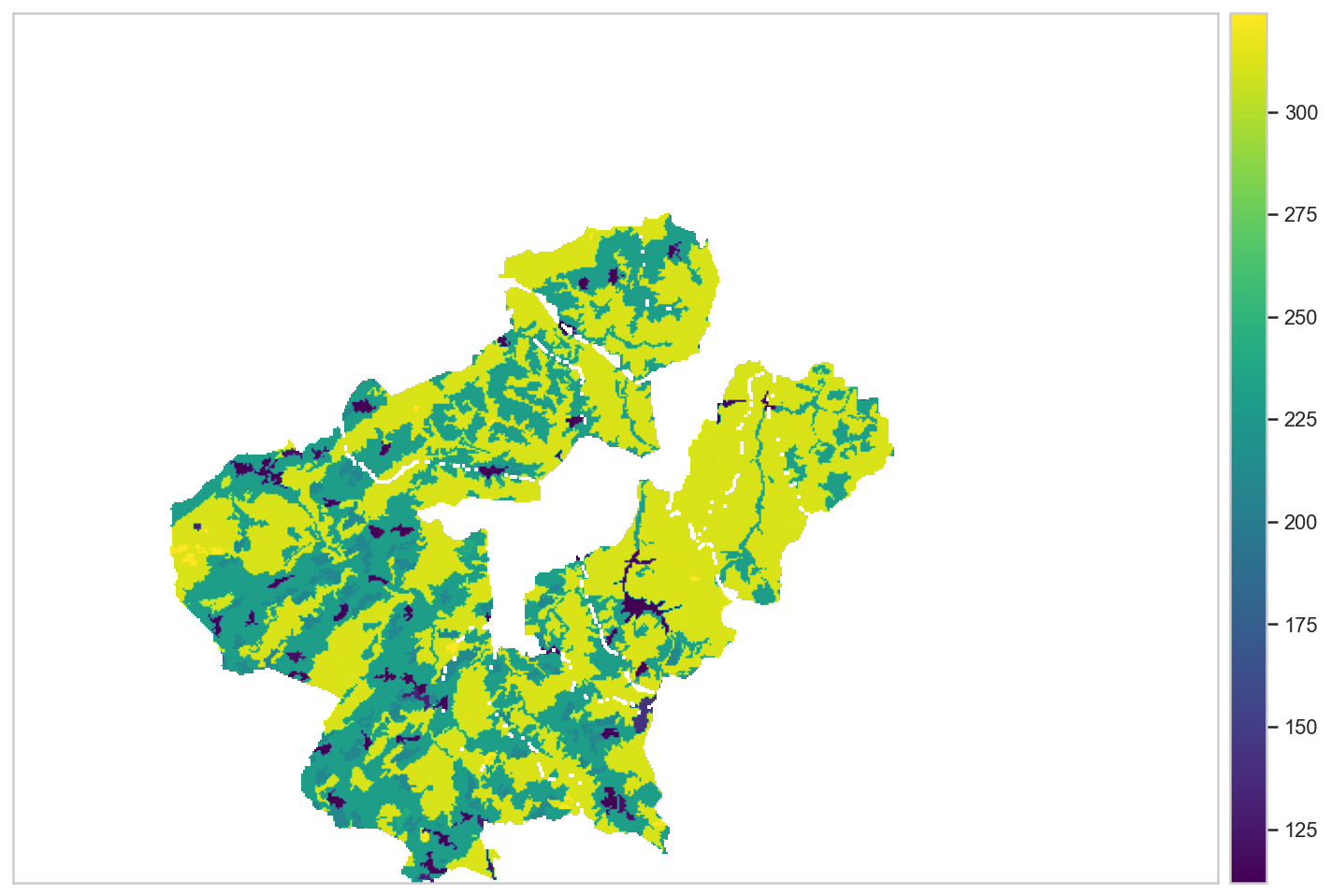
Landcover classification map Germany 2019

We looked up the land use for each deliniated watershed using as source the "classification map Germany 2019".

https://data.mundialis.de/geonetwork/srv/eng/catalog.search#/metadata/36512b46-f3aa-4aa4-8281-7584ec46c813

This landcover map was produced as an intermediate result in the course of the project incora (Inwertsetzung von Copernicus-Daten für die Raumbeobachtung, mFUND Förderkennzeichen: 19F2079C) in cooperation with ILS (Institut für Landes- und Stadtentwicklungsforschung gGmbH) and BBSR (Bundesinstitut für Bau-, Stadt- und Raumforschung) funded by BMVI (Federal Ministry of Transport and Digital Infrastructure). The goal of incora is an analysis of settlement and infrastructure dynamics in Germany based on Copernicus Sentinel data.

This classification is based on a time-series of monthly averaged, atmospherically corrected Sentinel-2 tiles (MAJA L3A-WASP: https://geoservice.dlr.de/web/maps/sentinel2:l3a:wasp; DLR (2019): Sentinel-2 MSI - Level 2A (MAJA-Tiles)- Germany). It consists of the following landcover classes:
10: forest
20: low vegetation
30: water
40: built-up
50: bare soil
60: agriculture

Out[42]:
2.46490
Out[7]:
geometry
0 POLYGON ((6.57550 50.42198, 6.57271 50.39538, ...
1 POLYGON ((6.92448 50.27242, 6.84534 50.27173, ...
2 POLYGON ((6.59683 50.43010, 6.61911 50.44731, ...
<class 'geopandas.geodataframe.GeoDataFrame'>
RangeIndex: 3 entries, 0 to 2
Data columns (total 1 columns):
 #   Column    Non-Null Count  Dtype   
---  ------    --------------  -----   
 0   geometry  3 non-null      geometry
dtypes: geometry(1)
memory usage: 152.0 bytes
Out[11]:
id left top right bottom geometry
0 1 326804.11 5.61e+06 367316.94 5.61e+06 LINESTRING (326804.106 5605381.555, 367316.937...
1 2 326804.11 5.61e+06 367316.94 5.61e+06 LINESTRING (326804.106 5605380.555, 367316.937...
2 3 326804.11 5.61e+06 367316.94 5.61e+06 LINESTRING (326804.106 5605379.555, 367316.937...
3 4 326804.11 5.61e+06 367316.94 5.61e+06 LINESTRING (326804.106 5605378.555, 367316.937...
4 5 326804.11 5.61e+06 367316.94 5.61e+06 LINESTRING (326804.106 5605377.555, 367316.937...
... ... ... ... ... ... ...
78956 78957 367312.11 5.61e+06 367312.11 5.57e+06 LINESTRING (367312.106 5605381.555, 367312.106...
78957 78958 367313.11 5.61e+06 367313.11 5.57e+06 LINESTRING (367313.106 5605381.555, 367313.106...
78958 78959 367314.11 5.61e+06 367314.11 5.57e+06 LINESTRING (367314.106 5605381.555, 367314.106...
78959 78960 367315.11 5.61e+06 367315.11 5.57e+06 LINESTRING (367315.106 5605381.555, 367315.106...
78960 78961 367316.11 5.61e+06 367316.11 5.57e+06 LINESTRING (367316.106 5605381.555, 367316.106...

78961 rows × 6 columns

Calculation was done by the Qgis Lecos module "patch stats" function. Here are only 3 of the 6 usage groups shown.

Out[18]:
Mid Ahr UpperAhr Armuthsbach Sahrbach Trierbach Adenauerbach Staffelbach Weidenbach Nohnerbach Liersbach Dennbach Wirftbach Ansbach
Land Use
agriculture 0.09 0.14 0.14 0.09 0.11 0.02 0.03 4.28e-03 0.15 0.04 3.30e-03 0.10 0.05
grass 0.30 0.40 0.32 0.26 0.36 0.22 0.26 1.76e-01 0.32 0.20 7.66e-02 0.31 0.24
forest 0.56 0.41 0.51 0.61 0.47 0.72 0.70 8.05e-01 0.49 0.74 9.06e-01 0.54 0.68

Corine land cover 2018 classification

The source file is big, and consists of land cover data of 39 European countries. I had to clip it.
Info about the 48 classes, and their colors: https://collections.sentinel-hub.com/corine-land-cover/readme.html

Out[2]:
900000.0
Out[8]:
(None,)
Out[9]:
<function DatasetReader.read_transform>
Out[10]:
[]
Out[14]:
(4031400.0, 2874100.0, 4283900.0, 3269900.0)
The crs of your data is: LOCAL_CS["ETRS_1989_LAEA",UNIT["metre",1,AUTHORITY["EPSG","9001"]],AXIS["Easting",EAST],AXIS["Northing",NORTH],AUTHORITY["EPSG","3035"]]
The nodatavalue of your data is: nan
The shape of your data is: (1, 3958, 2525)
The spatial resolution for your data is: (100.0, -100.0)
The metadata for your data is: {'RepresentationType': 'THEMATIC', 'scale_factor': 1.0, 'add_offset': 0.0}
Out[17]:
<AxesSubplot:>

Turns out that this data is not so fine gridded as the previous. However, the classification is very elaborate: there are 3 hierarchical levels.
But there are some "No data" patches, which are mostly (agricultural) land patches that appeared to have been plowed (Google maps), or left fallow, so the classification of these areas were too unclear at that time, I guess.

Get a Pandas dataframe from a PostgreSQL table using Psycopg2.

These are the Corine land cover percentages for the upper Ahr area.

Out[38]:
Value Number Percent clc_legend_GRID_CODE clc_legend_LABEL1 clc_legend_LABEL2 clc_legend_LABEL3
0 112 916 0.036325 2 Artificial surfaces Urban fabric Discontinuous urban fabric
1 121 71 0.002816 3 Artificial surfaces Industrial, commercial and transport units Industrial or commercial units
2 122 28 0.001110 4 Artificial surfaces Industrial, commercial and transport units Road and rail networks and associated land
3 131 120 0.004759 7 Artificial surfaces Mine, dump and construction sites Mineral extraction sites
4 133 2 0.000079 9 Artificial surfaces Mine, dump and construction sites Construction sites
5 211 2129 0.084427 12 Agricultural areas Arable land Non-irrigated arable land
6 231 11833 0.469247 18 Agricultural areas Pastures Pastures
7 242 61 0.002419 20 Agricultural areas Heterogeneous agricultural areas Complex cultivation patterns
8 243 39 0.001547 21 Agricultural areas Heterogeneous agricultural areas Land principally occupied by agriculture, with...
9 311 4155 0.164770 23 Forest and semi natural areas Forests Broad-leaved forest
10 312 4196 0.166396 24 Forest and semi natural areas Forests Coniferous forest
11 313 1497 0.059365 25 Forest and semi natural areas Forests Mixed forest
12 321 29 0.001150 26 Forest and semi natural areas Scrub and/or herbaceous vegetation associations Natural grasslands
13 324 141 0.005591 29 Forest and semi natural areas Scrub and/or herbaceous vegetation associations Transitional woodland-shrub

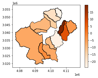
The proportions of the 2 classifications turn out to be the same for forests, but not at all for other classes.

  • The amount of grassland has been captured under the Corine-term 'Pastures', and meanwhile
  • the amount of the term "Natural grasslands" has been rendered neglictable by classification rules
  • the no-data patches raised the amount of builded area from 2,8 to 3,6%.

There seems to be some unification feasable with the up todate German map by only using the coarser level 2 labels.

7.20893646 9.190225000000002 1.274837842030307

Here we clip the raster to the extend of our area of interest.

Out[22]:
(4068937.4749, 3019512.9211000004, 4134313.9289000006, 3066728.0581)
The crs of your data is: LOCAL_CS["ETRS89-extended / LAEA Europe",UNIT["metre",1,AUTHORITY["EPSG","9001"]],AXIS["Easting",EAST],AXIS["Northing",NORTH],AUTHORITY["EPSG","3035"]]
The nodatavalue of your data is: nan
The shape of your data is: (1, 472, 654)
The spatial resolution for your data is: (99.9639969418966, -100.03206991525445)
The metadata for your data is: {'STATISTICS_MAXIMUM': 324, 'STATISTICS_MEAN': 271.22897027616, 'STATISTICS_MINIMUM': 112, 'STATISTICS_STDDEV': 49.628820944876, 'STATISTICS_VALID_PERCENT': 22.44, 'scale_factor': 1.0, 'add_offset': 0.0}

It seems that we clipped on an extend, not by the mask layer. So we'll make corrections to the results.

Forest/Non-forest map of 2015

The TanDEM-X Forest/Non-Forest Map (FNF) has been generated by processing and mosaicking more than 500,000 TanDEM-X bistatic images acquired from 2011 until 2015. The map has a spatial resolution of 50 x 50m.

We note that the data is rather old. Especially considering the damage caused to coniferous trees by the progress of the spruce beetle, and the mandatory affected tree fellings.

A comparison of the forest area land cover between 2015 and 2019-2020 can be made:

c:\program files\python38\lib\site-packages\geopandas\_compat.py:111: UserWarning: The Shapely GEOS version (3.8.1-CAPI-1.13.3) is incompatible with the GEOS version PyGEOS was compiled with (3.10.0-CAPI-1.16.0). Conversions between both will be slow.
  warnings.warn(
Out[1]:
Name Forests201 Forests2_1 Forests2_2 geometry
0 Nohnerbach 73.0 160289.0 157178.0 POLYGON ((4092905.838 3032622.965, 4092900.727...
1 Vischelbach 2609.0 69178.0 116361.0 POLYGON ((4104826.147 3050124.935, 4104806.467...
2 Liersbach 47.0 63939.0 198892.0 POLYGON ((4098323.022 3050116.109, 4098496.509...
3 Ansbach 0.0 46359.0 100612.0 POLYGON ((4090406.748 3042084.416, 4090434.837...
4 Staffelbach 3476.0 111471.0 254536.0 POLYGON ((4110741.362 3042486.748, 4110739.617...
5 Wirftbach 0.0 113959.0 135075.0 POLYGON ((4101582.244 3029538.684, 4101562.486...
6 Dennbach 0.0 17403.0 173607.0 POLYGON ((4105954.626 3038316.732, 4105625.973...
7 Weidenbach 1323.0 72796.0 297869.0 POLYGON ((4108346.571 3034851.978, 4108095.028...
8 Adenauerbach 1712.0 140335.0 426602.0 POLYGON ((4103890.613 3029795.294, 4103259.401...
9 Trierbach 4573.0 290381.0 258336.0 POLYGON ((4095046.191 3031950.278, 4095317.435...
10 Upper Ahr 16600.0 1484399.0 1020503.0 POLYGON ((4096023.071 3022630.947, 4096002.967...
11 Sahrbach 0.0 190453.0 269934.0 POLYGON ((4100654.057 3048603.390, 4100654.688...
12 Armuthsbach 4664.0 351770.0 370654.0 POLYGON ((4086674.715 3044973.492, 4087231.756...
Out[2]:
Name Forests201 Forests2_1 Forests2_2 geometry
0 Nohnerbach 0.0 156931.0 160609.0 POLYGON ((4092905.838 3032622.965, 4092900.727...
1 Vischelbach 0.0 55652.0 132496.0 POLYGON ((4104826.147 3050124.935, 4104806.467...
2 Liersbach 0.0 56573.0 206305.0 POLYGON ((4098323.022 3050116.109, 4098496.509...
3 Ansbach 0.0 42579.0 104392.0 POLYGON ((4090406.748 3042084.416, 4090434.837...
4 Staffelbach 98.0 107002.0 262383.0 POLYGON ((4110741.362 3042486.748, 4110739.617...
5 Wirftbach 0.0 103312.0 145722.0 POLYGON ((4101582.244 3029538.684, 4101562.486...
6 Dennbach 0.0 21751.0 169259.0 POLYGON ((4105954.626 3038316.732, 4105625.973...
7 Weidenbach 0.0 78423.0 293565.0 POLYGON ((4108346.571 3034851.978, 4108095.028...
8 Adenauerbach 0.0 114086.0 454563.0 POLYGON ((4103890.613 3029795.294, 4103259.401...
9 Trierbach 0.0 271938.0 281352.0 POLYGON ((4095046.191 3031950.278, 4095317.435...
10 Upper Ahr 22.0 1390044.0 1131436.0 POLYGON ((4096023.071 3022630.947, 4096002.967...
11 Sahrbach 0.0 162261.0 298126.0 POLYGON ((4100654.057 3048603.390, 4100654.688...
12 Armuthsbach 0.0 322252.0 404836.0 POLYGON ((4086674.715 3044973.492, 4087231.756...

Percentage of forest that were lost, or gained (-), between 2015 and 2019.

Out[13]:
Pct_forest_loss Pct_nonforest_loss geometry
Name
Nohnerbach 2.136244 -2.139794 POLYGON ((4092905.838 3032622.965, 4092900.727...
Vischelbach 12.177726 -24.304607 POLYGON ((4104826.147 3050124.935, 4104806.467...
Liersbach 3.593224 -13.020345 POLYGON ((4098323.022 3050116.109, 4098496.509...
Ansbach 3.620967 -8.877616 POLYGON ((4090406.748 3042084.416, 4090434.837...
Staffelbach 2.990666 -4.176557 POLYGON ((4110741.362 3042486.748, 4110739.617...
Wirftbach 7.306378 -10.305676 POLYGON ((4101582.244 3029538.684, 4101562.486...
Dennbach -2.568844 19.989886 POLYGON ((4105954.626 3038316.732, 4105625.973...
Weidenbach -1.466115 7.175191 POLYGON ((4108346.571 3034851.978, 4108095.028...
Adenauerbach 6.151183 -23.008082 POLYGON ((4103890.613 3029795.294, 4103259.401...
Trierbach 8.180500 -6.782061 POLYGON ((4095046.191 3031950.278, 4095317.435...
Upper Ahr 9.804620 -6.787915 POLYGON ((4096023.071 3022630.947, 4096002.967...
Sahrbach 9.456404 -17.374477 POLYGON ((4100654.057 3048603.390, 4100654.688...
Armuthsbach 8.443419 -9.159912 POLYGON ((4086674.715 3044973.492, 4087231.756...

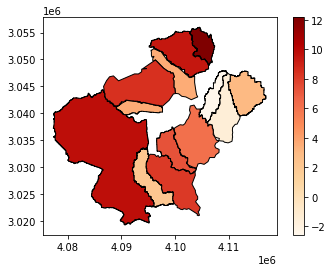
The main causes for concern were indeed: Upper Ahrregion, Sahrbach, Trierbach, Armuthsbach and Vischelbach.

Incorporation of the travel time of the flows.

It takes some time for the outflow of a specific tributary to reach Altenahr. First I applied a linear method, however a flood wave has an flow acceleration in respect of time. Hence a complicated nonlinear method should be used later. How complicated this implementation is, is the fact that this flow acceleration is not included in the HEC-RAS software flood wave module.
Here I tried out an approximation:

Out[26]:
Time
2021-07-07 00:00:00   2021-07-07 00:15:00
2021-07-07 00:15:00   2021-07-07 00:30:00
2021-07-07 00:30:00   2021-07-07 00:45:00
2021-07-07 00:45:00   2021-07-07 01:00:00
2021-07-07 01:00:00   2021-07-07 01:15:00
                              ...        
2021-07-24 11:15:00   2021-07-24 11:30:00
2021-07-24 11:30:00   2021-07-24 11:45:00
2021-07-24 11:45:00   2021-07-24 12:00:00
2021-07-24 12:00:00   2021-07-24 12:15:00
2021-07-24 12:15:00   2021-07-24 12:30:00
Name: Time_lag, Length: 1682, dtype: datetime64[ns]
Out[27]:
['Sahr',
 'Liers',
 'Armuths',
 'Ans',
 'Nohner',
 'Trier',
 'Wirft',
 'Adenauer',
 'Denn',
 'Staffel',
 'Vischel',
 'UpperAhr',
 'Weidenbach']

Estimation of the length of the waterpaths from outlet point to Altenahr. The small error to consider is that the location of the outlet point and the location of the respective measurestation are not same.

Out[5]:
[('Sahr', 2.17, 50.51086115566, 6.974915458214),
 ('Liers', 10, 50.459138381369975, 6.944930767512368),
 ('Armuths', 18.8, 50.450921792969, 6.8691766649903),
 ('Ans', 22, 50.432569232799295, 6.854819103572359),
 ('Nohner', 35.5, 50.362390498191665, 6.828113687373144),
 ('Trier', 34, 50.36310517182589, 6.83067860787267),
 ('Wirft', 22, 50.37133200617, 6.8429410315291745),
 ('Adenauer', 11.2, 50.44348104478261, 6.933994595890211),
 ('Denn', 6.3, 50.47694306572389, 6.986004732775374),
 ('Staffel', 8.8, 50.48225212686384, 7.062665427811296),
 ('Vischel', 11.2, 50.51162208518743, 6.976000717336059),
 ('UpperAhr', 1, 50.38235, 6.80951)]

Distances of the outlet points to Altenahr, and their Latitude and Longitude.

Map for location of the main tributary outletpoints of the Ahr

First I estimated the water speed during the flood 9 km/ hour, but this might be only true for the max. discharge, or with acceleration included.
In physics the speed of a sudden flood water wave peak is $c_{hw}$.

Out[60]:
8.123702693633332
per minut  100.0 150.0 c_hw: 8.123702693633332

We only need the trajectory from source downstream (or Müsch) to Altenahr. Moreover the streettunnel at Altenahr was from a certain level (and point in time) an artificial bypass for a portion of the flood water.
The difference in elevation, or slope, is +- 0.4%...

Out[19]:
0.00402

Starting the flow model with a simplification:

There is no elongation (diffusion) or shortening (dynamic) of the wave.

We can use Mannings formula for calculating the water velocity, with a hydraulic radius $R_h$, $V_w$ in m/s, flowing though a rough natural stream channel.
Channels in coarse gravel: n= 0.028
Also using an extra penalty for the "n" coefficient due to

  • Relative effect of obstructions: buildings and bridges on the flowpath.
    • Severe 0.040 to 0.060 - Large and small sections alternating
  • frequently or shape changes causing frequent shifting of main flow from side-to-side:
    • 0.010 to 0.015
  • Degree of irregularity:
    • severe : 0.02
  • Vegetation and flow conditions comparable to:
    • Growing season; trees intergrown with weeds and brush, all in full foliage... Very high: 0.05-0.10
  • degree of meandering: > 1.5: Severe
    • modifying value 0.30 * $n_s$
Out[25]:
1.73254
Out[16]:
0.06690

The speed of the water of that flow: $u=\frac {1}{n_m}h^{2/3}\sqrt S$

Out[12]:
11.721039594098983
Out[20]:
2.8052860392611754
Out[21]:
1.8869637035389073
Out[22]:
113.21782221233444
Out[23]:
6.793069332740067

Penalty for blocking flow path by clogged bridges

Out[24]:
8.262842515642008
Out[25]:
137.7140419273668
Out[34]:
261.53210
Out[35]:
15.69193

Wave Celerity of sudden floodwave

  • The floodwave celerity c is always faster than the flow velocity when 𝛽 >1 (𝛽V=c)
  • Floodwave celerity increases with flow depth
    • Larger floodwaves (larger flow depth) propagate faster than small floodwaves
    • Cause nonlinearity in the downstream propagation of floodwaves
    • Linear techniques based on superposition fail to adequately simulate floodwave propagation in channels
    • Method of isochrons used in hydrology is not applicable to both small and large floodwaves
  • The value of 𝛽 and flow velocity will affect the arrival of a flood peak.
Out[28]:
Stream Bach Distance Lati Long Latitude Longitude Streamcode
0 Sahr Sahrbach 2.17 50.51 6.97 50.54 6.85 27188
1 Liers Liersbach 10.00 50.46 6.94 50.53 6.83 271872
2 Armuths Armuthsbach 18.80 50.45 6.87 50.47 6.71 271856
3 Ans Ansbach 22.00 50.43 6.85 50.44 6.75 271854
4 Nohner Nohnerbach 35.50 50.36 6.83 50.28 6.88 271812
5 Trier Trierbach 34.00 50.36 6.83 50.30 6.91 27184
6 Wirft Wirftbach 22.00 50.37 6.84 50.34 6.93 271899
7 Adenauer Adenauerbach 11.20 50.44 6.93 50.35 6.97 27186
8 Denn Dennbach 6.30 50.48 6.99 50.42 6.97 2718748
9 Staffel Staffelbach 10.20 50.48 7.03 50.46 7.11 271874
10 Vischel Vischelbach 1.00 50.51 6.98 50.57 6.94 271892
11 Weiden Weidenbach 8.30 50.48 7.02 50.39 7.03 2718741
12 UpperAhr UpperAhr 34.20 50.38 6.81 50.44 6.65 27182
Out[9]:
0      20.0
1      92.0
2     172.0
3     201.0
4     325.0
5     311.0
6     201.0
7     103.0
8      58.0
9      81.0
10      9.0
11    103.0
12    313.0
Name: km, dtype: float64
Out[29]:
0      16.0
1      72.0
2     136.0
3     159.0
4     257.0
5     246.0
6     159.0
7      81.0
8      46.0
9      74.0
10      7.0
11     60.0
12    248.0
Name: km, dtype: float64

We apply the estimated time it takes for the water of the different outlets to travel to Altenahr.

The time it takes for the water to travel to Altenahr is included in the new index.

Out[32]:
Flow rate (m³/s)
Time_lag
2021-07-13 01:12:00 0.0
2021-07-13 01:27:00 0.0
2021-07-13 01:42:00 0.0
2021-07-13 01:57:00 0.0
2021-07-13 02:12:00 0.0
... ...
2021-10-13 14:27:00 0.0
2021-10-13 14:42:00 0.0
2021-10-13 14:57:00 0.0
2021-10-13 15:12:00 0.0
2021-10-13 15:27:00 0.0

8890 rows × 1 columns

Out[34]:
Flow rate (m³/s)Sahr Flow rate (m³/s)Liers
Time_lag
2021-07-07 00:16:00 0.0 NaN
2021-07-07 00:31:00 0.0 NaN
2021-07-07 00:46:00 0.0 NaN
2021-07-07 01:01:00 0.0 NaN
2021-07-07 01:16:00 0.0 NaN
... ... ...
2021-10-13 14:27:00 NaN 0.0
2021-10-13 14:42:00 NaN 0.0
2021-10-13 14:57:00 NaN 0.0
2021-10-13 15:12:00 NaN 0.0
2021-10-13 15:27:00 NaN 0.0

10572 rows × 2 columns

<class 'pandas.core.frame.DataFrame'>
DatetimeIndex: 10572 entries, 2021-07-07 00:16:00 to 2021-10-13 15:27:00
Data columns (total 2 columns):
 #   Column                 Non-Null Count  Dtype  
---  ------                 --------------  -----  
 0   Flow rate (m³/s)Sahr   1682 non-null   float64
 1   Flow rate (m³/s)Liers  8890 non-null   float64
dtypes: float64(2)
memory usage: 247.8 KB
Out[36]:
Flow rate (m³/s)Sahr Flow rate (m³/s)Liers Flow rate (m³/s) Flow rate (m³/s)Ans Flow rate (m³/s)Nohner Flow rate (m³/s)Trier Flow rate (m³/s)Wirft Flow rate (m³/s)Adenauer
Time_lag
2021-06-10 01:21:00 NaN NaN NaN NaN NaN NaN NaN 0.0
2021-06-10 02:21:00 NaN NaN NaN NaN NaN NaN NaN 0.0
2021-06-10 03:21:00 NaN NaN NaN NaN NaN NaN NaN 0.0
2021-06-10 04:21:00 NaN NaN NaN NaN NaN NaN NaN 0.0
2021-06-10 05:21:00 NaN NaN NaN NaN NaN NaN NaN 0.0
... ... ... ... ... ... ... ... ...
2021-10-13 16:54:00 NaN NaN NaN 0.0 NaN NaN NaN NaN
2021-10-13 17:09:00 NaN NaN NaN 0.0 NaN NaN NaN NaN
2021-10-13 17:16:00 NaN NaN 0.0 NaN NaN NaN NaN NaN
2021-10-13 17:24:00 NaN NaN NaN 0.0 NaN NaN NaN NaN
2021-10-13 17:39:00 NaN NaN NaN 0.0 NaN NaN NaN NaN

23181 rows × 8 columns

Out[37]:
Flow rate (m³/s)Sahr Flow rate (m³/s)Liers Flow rate (m³/s) Flow rate (m³/s)Ans Flow rate (m³/s)Nohner Flow rate (m³/s)Trier Flow rate (m³/s)Wirft Flow rate (m³/s)Adenauer Flow rate (m³/s)Denn Flow rate (m³/s)Staffel Flow rate (m³/s)Vischel Flow rate (m³/s)UpperAhr
Time_lag
2021-06-10 00:46:00 NaN NaN NaN NaN NaN NaN NaN NaN 0.0 NaN NaN NaN
2021-06-10 01:01:00 NaN NaN NaN NaN NaN NaN NaN NaN 0.0 NaN NaN NaN
2021-06-10 01:16:00 NaN NaN NaN NaN NaN NaN NaN NaN 0.0 NaN NaN NaN
2021-06-10 01:21:00 NaN NaN NaN NaN NaN NaN NaN 0.0 NaN NaN NaN NaN
2021-06-10 01:31:00 NaN NaN NaN NaN NaN NaN NaN NaN 0.0 NaN NaN NaN
... ... ... ... ... ... ... ... ... ... ... ... ...
2021-10-13 16:54:00 NaN NaN NaN 0.0 NaN NaN NaN NaN NaN NaN NaN NaN
2021-10-13 17:09:00 NaN NaN NaN 0.0 NaN NaN NaN NaN NaN NaN NaN NaN
2021-10-13 17:16:00 NaN NaN 0.0 NaN NaN NaN NaN NaN NaN NaN NaN NaN
2021-10-13 17:24:00 NaN NaN NaN 0.0 NaN NaN NaN NaN NaN NaN NaN NaN
2021-10-13 17:39:00 NaN NaN NaN 0.0 NaN NaN NaN NaN NaN NaN NaN NaN

28375 rows × 12 columns

Next we replace the nan's in the end, and resample to 15 minute bins so we are in sync with the measurement rate...

Out[40]:
Flow rate (m³/s)Sahr Flow rate (m³/s)Liers Flow rate (m³/s) Flow rate (m³/s)Ans Flow rate (m³/s)Nohner Flow rate (m³/s)Trier Flow rate (m³/s)Wirft Flow rate (m³/s)Adenauer Flow rate (m³/s)Denn Flow rate (m³/s)Staffel Flow rate (m³/s)Vischel Flow rate (m³/s)UpperAhr
Time_lag
2021-06-10 00:46:00 0.0 0.0 0.0 0.0 0.0 0.0 0.0 0.0 0.0 0.0 0.0 0.0
2021-06-10 01:01:00 0.0 0.0 0.0 0.0 0.0 0.0 0.0 0.0 0.0 0.0 0.0 0.0
2021-06-10 01:16:00 0.0 0.0 0.0 0.0 0.0 0.0 0.0 0.0 0.0 0.0 0.0 0.0
2021-06-10 01:21:00 0.0 0.0 0.0 0.0 0.0 0.0 0.0 0.0 0.0 0.0 0.0 0.0
2021-06-10 01:31:00 0.0 0.0 0.0 0.0 0.0 0.0 0.0 0.0 0.0 0.0 0.0 0.0
... ... ... ... ... ... ... ... ... ... ... ... ...
2021-10-13 16:54:00 0.0 0.0 0.0 0.0 0.0 0.0 0.0 0.0 0.0 0.0 0.0 0.0
2021-10-13 17:09:00 0.0 0.0 0.0 0.0 0.0 0.0 0.0 0.0 0.0 0.0 0.0 0.0
2021-10-13 17:16:00 0.0 0.0 0.0 0.0 0.0 0.0 0.0 0.0 0.0 0.0 0.0 0.0
2021-10-13 17:24:00 0.0 0.0 0.0 0.0 0.0 0.0 0.0 0.0 0.0 0.0 0.0 0.0
2021-10-13 17:39:00 0.0 0.0 0.0 0.0 0.0 0.0 0.0 0.0 0.0 0.0 0.0 0.0

28375 rows × 12 columns

resample into 15 or 5 minute bins.

Out[44]:
Time_lag
2021-06-10 00:45:00    0.0
2021-06-10 01:00:00    0.0
2021-06-10 01:15:00    0.0
2021-06-10 01:30:00    0.0
2021-06-10 01:45:00    0.0
                      ... 
2021-10-13 16:30:00    0.0
2021-10-13 16:45:00    0.0
2021-10-13 17:00:00    0.0
2021-10-13 17:15:00    0.0
2021-10-13 17:30:00    0.0
Freq: 15T, Name: Sum, Length: 12068, dtype: float64

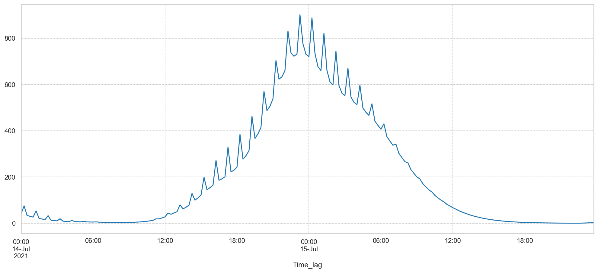
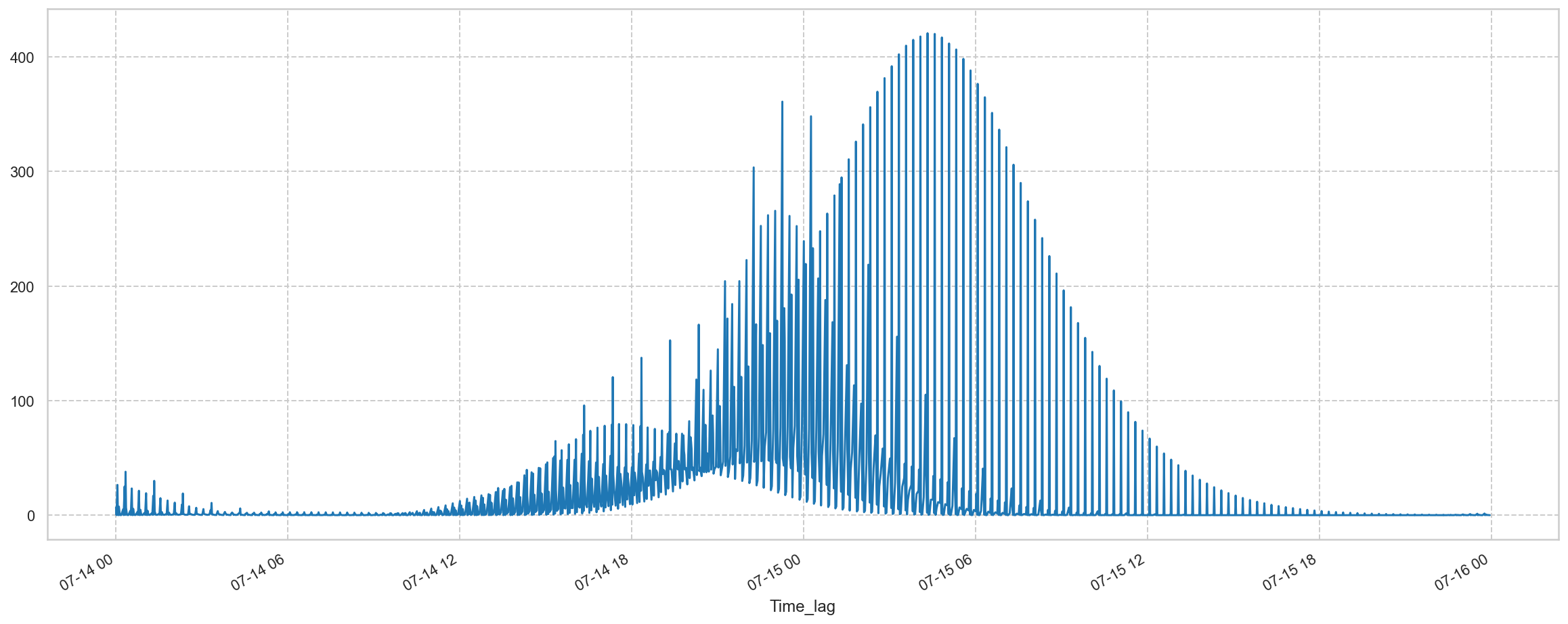
The jagged form of the curve is caused by the fact that some rainfall data was 60 minute interval, but 15 minutes for the outflows (before time shifts).

Measured outflow and water level at Müsch

Müsch is the place where the outflows of upper Ahr streams and those of Trierbach and Nohnerbach combine.

<class 'pandas.core.frame.DataFrame'>
Int64Index: 775 entries, 0 to 774
Data columns (total 2 columns):
 #   Column           Non-Null Count  Dtype         
---  ------           --------------  -----         
 0   Datum            775 non-null    datetime64[ns]
 1   Abfluss in m3/s  775 non-null    float64       
dtypes: datetime64[ns](1), float64(1)
memory usage: 18.2 KB
Out[50]:
Abfluss in m3/s
Datum
2021-07-07 11:45:00 2.00
2021-07-07 12:00:00 2.00
2021-07-07 12:15:00 2.00
2021-07-07 12:30:00 2.00
2021-07-07 12:45:00 2.00
... ...
2021-07-15 12:15:00 114.66
2021-07-15 12:30:00 112.06
2021-07-15 12:45:00 108.26
2021-07-15 13:00:00 108.26
2021-07-15 13:15:00 104.57

775 rows × 1 columns

<class 'pandas.core.frame.DataFrame'>
DatetimeIndex: 775 entries, 2021-07-07 11:45:00 to 2021-07-15 13:15:00
Data columns (total 1 columns):
 #   Column           Non-Null Count  Dtype  
---  ------           --------------  -----  
 0   Abfluss in m3/s  775 non-null    float64
dtypes: float64(1)
memory usage: 28.3 KB
Out[51]:
Datum Abfluss in m3/s
0 2021-07-07 11:45:00 2.0
1 2021-07-07 12:00:00 2.0
2 2021-07-07 12:15:00 2.0
Out[70]:
Flow rate (m³/s)
Time
2021-07-12 00:00:00 0.00e+00
2021-07-12 00:15:00 0.00e+00
2021-07-12 00:30:00 0.00e+00
2021-07-12 00:45:00 0.00e+00
2021-07-12 01:00:00 0.00e+00
... ...
2021-07-17 03:15:00 4.42e-06
2021-07-17 03:30:00 0.00e+00
2021-07-17 03:45:00 0.00e+00
2021-07-17 04:00:00 0.00e+00
2021-07-17 04:15:00 0.00e+00

498 rows × 1 columns

Out[71]:
Flow rate (m³/s)
Time
2021-07-14 18:00:00 129.74
2021-07-14 18:15:00 138.73
2021-07-14 18:30:00 148.45
2021-07-14 18:45:00 158.80
2021-07-14 19:00:00 169.72
2021-07-14 19:15:00 180.65
2021-07-14 19:30:00 192.60
2021-07-14 19:45:00 205.50
2021-07-14 20:00:00 219.24
2021-07-14 20:15:00 232.98
2021-07-14 20:30:00 247.81
2021-07-14 20:45:00 263.20
2021-07-14 21:00:00 278.99
2021-07-14 21:15:00 294.78
2021-07-14 21:30:00 310.57
2021-07-14 21:45:00 326.01
2021-07-14 22:00:00 341.02
2021-07-14 22:15:00 356.04
2021-07-14 22:30:00 369.51
2021-07-14 22:45:00 381.40
2021-07-14 23:00:00 391.79
2021-07-14 23:15:00 402.17
2021-07-14 23:30:00 409.70
2021-07-14 23:45:00 414.79
2021-07-15 00:00:00 417.70
2021-07-15 00:15:00 420.60
2021-07-15 00:30:00 419.99
2021-07-15 00:45:00 416.86
2021-07-15 01:00:00 411.62
<class 'pandas.core.frame.DataFrame'>
DatetimeIndex: 498 entries, 2021-07-12 04:05:00 to 2021-07-17 08:20:00
Data columns (total 1 columns):
 #   Column            Non-Null Count  Dtype  
---  ------            --------------  -----  
 0   Flow rate (m³/s)  498 non-null    float64
dtypes: float64(1)
memory usage: 23.9 KB
Out[74]:
Flow rate (m³/s) Abfluss in m3/s
2021-07-12 00:00:00 0.00 2.78
2021-07-12 00:15:00 0.00 2.78
2021-07-12 00:30:00 0.00 2.78
2021-07-12 00:45:00 0.00 2.78
2021-07-12 01:00:00 0.00 2.78
... ... ...
2021-07-15 12:15:00 9.02 114.66
2021-07-15 12:30:00 7.92 112.06
2021-07-15 12:45:00 6.97 108.26
2021-07-15 13:00:00 6.15 108.26
2021-07-15 13:15:00 5.33 104.57

342 rows × 2 columns

Out[83]:
Time
2021-07-14 10:00:00      0.52
2021-07-14 10:15:00      0.55
2021-07-14 10:30:00      0.66
2021-07-14 10:45:00      0.84
2021-07-14 11:00:00      1.09
                        ...  
2021-07-15 05:00:00    196.19
2021-07-15 05:15:00    181.48
2021-07-15 05:30:00    167.72
2021-07-15 05:45:00    154.74
2021-07-15 06:00:00    142.48
Name: Flow rate (m³/s), Length: 81, dtype: float64
Out[84]:
Time_lag
2021-07-14 10:02:00     0.09
2021-07-14 10:17:00     0.08
2021-07-14 10:32:00     0.06
2021-07-14 10:47:00     0.05
2021-07-14 11:02:00     0.04
                       ...  
2021-07-15 04:47:00    31.37
2021-07-15 05:02:00    28.62
2021-07-15 05:17:00    25.94
2021-07-15 05:32:00    23.36
2021-07-15 05:47:00    20.92
Name: Flow rate (m³/s), Length: 80, dtype: float64
Out[85]:
2021-07-12 00:00:00   NaN
2021-07-12 00:15:00   NaN
2021-07-12 00:30:00   NaN
2021-07-12 00:45:00   NaN
2021-07-12 01:00:00   NaN
                       ..
2021-07-17 06:32:00   NaN
2021-07-17 06:47:00   NaN
2021-07-17 07:02:00   NaN
2021-07-17 07:17:00   NaN
2021-07-17 07:32:00   NaN
Name: Flow rate (m³/s), Length: 896, dtype: float64
Out[86]:
Time
2021-07-14 10:00:00      1.05
2021-07-14 10:15:00      1.33
2021-07-14 10:30:00      1.82
2021-07-14 10:45:00      2.47
2021-07-14 11:00:00      3.32
                        ...  
2021-07-15 05:00:00    199.40
2021-07-15 05:15:00    184.16
2021-07-15 05:30:00    169.95
2021-07-15 05:45:00    156.61
2021-07-15 06:00:00    144.03
Name: Flow rate (m³/s), Length: 81, dtype: float64

Around 14-07-2021 14:00 the Müsch sensor gave "strange" values, so they (HVZ) switched to the backup sensor. This one also gave odd results.
A copy of the recorded values that day has been provided, and I obtained a copy of the records.
I suspected that the flood forces discalibrated the sensors in their final moments. They should anytime be able to measure the correct waterlevel, also in the case of an extreme highwater event. This calculation is based on a fixed Pegelnullpunkt, in this case 292.77 m asl.

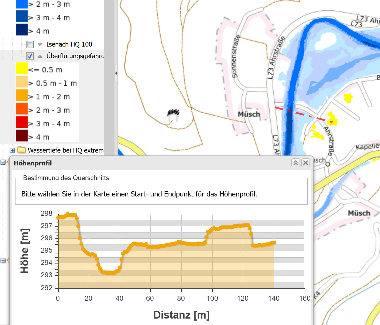
Flood water bypass over the eastbank

After some time I got more info to find reasons for the "strange" water level values:

  • Ultrasonic and radar sensors have a blind range of 15 to 150 cm, where they have difficulties correctly measuring heights.
    • They were placed too low for water levels during torrential floods.
    • Floating debris in the flood water adds to the problem.
  • When you see the elevation profile with the water flow path, you can deduct some things:

    • Above 2.9 m the water mass can stream over the eastbank, so that reduces the water level. It is visible as a plateau in the orange curve.

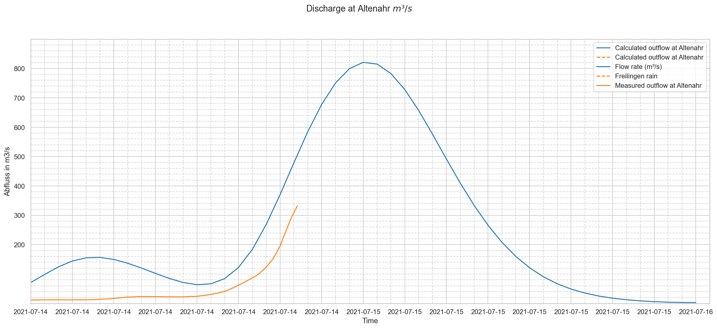
Measured outflow and water level at Altenahr:

Out[88]:
Datum
2021-07-12 00:00:00    6.25
2021-07-12 00:15:00    6.25
2021-07-12 00:30:00    6.25
2021-07-12 00:45:00    6.25
2021-07-12 01:00:00    6.25
2021-07-12 01:15:00    6.25
2021-07-12 01:30:00    6.25
2021-07-12 01:45:00    6.25
2021-07-12 02:00:00    6.25
2021-07-12 02:15:00    5.98
Name: Abfluss in m3/s, dtype: float64
Out[89]:
Datum
2021-06-24 17:15:00    59.0
2021-06-24 17:30:00    60.0
2021-06-24 17:45:00    60.0
2021-06-24 18:00:00    60.0
2021-06-24 18:15:00    60.0
2021-06-24 18:30:00    60.0
2021-06-24 18:45:00    61.0
2021-06-24 19:00:00    62.0
2021-06-24 19:15:00    62.0
2021-06-24 19:30:00    62.0
Name: Wasserstand in cm, dtype: float64

Fine gridded plot with time shifted, calculated discharges at Altenahr:

Note: the "Measured outflow at Altenahr", provided by the RLP Umwelt services, is derived from the water level.
The discharges were calculated by Lekan, and time shifted with a time lag in correspondence with the distance to Altenahr hydrometerstation.

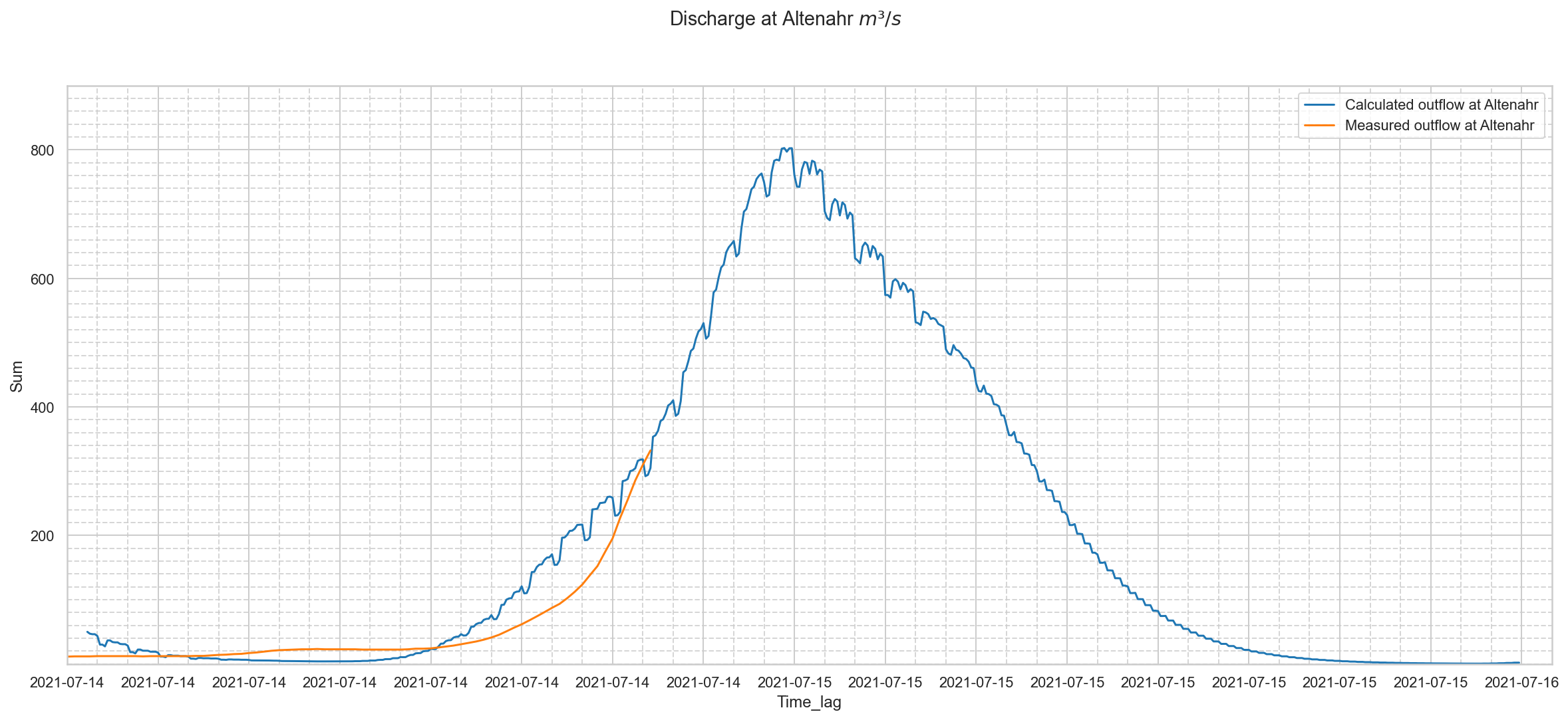
This plot was based on a former calculation with coarser rainfall data...

The rainfall timeseries were not logged in European summer timings, so that means that an event at 18:00 is in fact happening at 19:00.
In other words: the blue curve has to move 1 hour to the right to be in sync with the waterlevel/outflow readings, which were in summer timings.

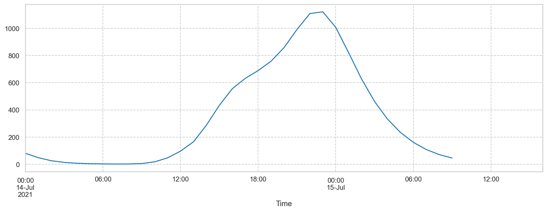
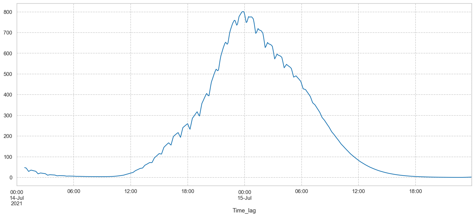
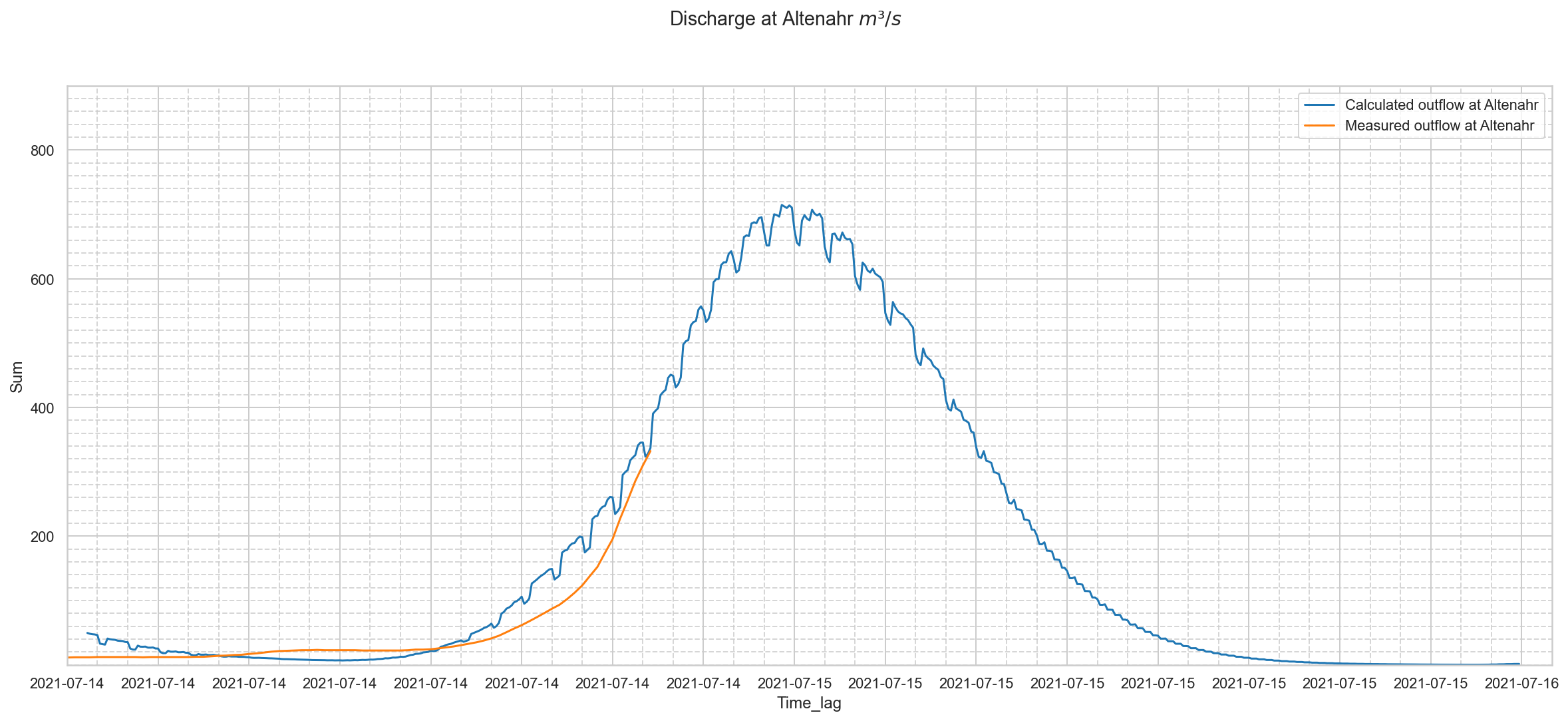
Compare the combined outflows of the upper and mid section of the Ahr drainage area with the derived outflow at Altenahr.

  • The "derived" outflow means the debit based on the measured water levels, which is incorrect during floods due to the phenomenon of hysteresis.
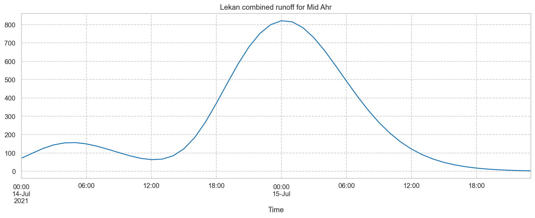
  • The combined outflow was calculated by the program "Lekan", based on 13 main tributaries.
    • Peak factor was changed: 484 to 600, as it seems more appropriate in this mountainous valley.
  • Curve numbers were assigned based on the proportion of the land use area in the catchments.
    • Qgis was used to calculate these land use proportions of forest, grassland, agricultural land, buildup area and vegetationless soil.
    • Qgis was used to find the hydrological soil groups, which where group C, and <10% C/d (lower drainage level)
  • Applied was an small penalty - because of the high wetness of the soils at 13/07 - for the curve numbers.

Source: Germany 2019 – Land cover based on Sentinel-2 data

Out[99]:
Flow rate (m³/s) Freilingen rain
Time
2021-07-14 00:00:00 71.01 NaN
2021-07-14 01:00:00 98.23 NaN
2021-07-14 02:00:00 124.31 NaN
Out[96]:
Flow rate (m³/s) Freilingen rain Abfluss in m3/s
2021-07-14 00:00:00 71.01 NaN 11.33
2021-07-14 01:00:00 98.23 NaN 12.07
2021-07-14 02:00:00 124.31 NaN 12.07

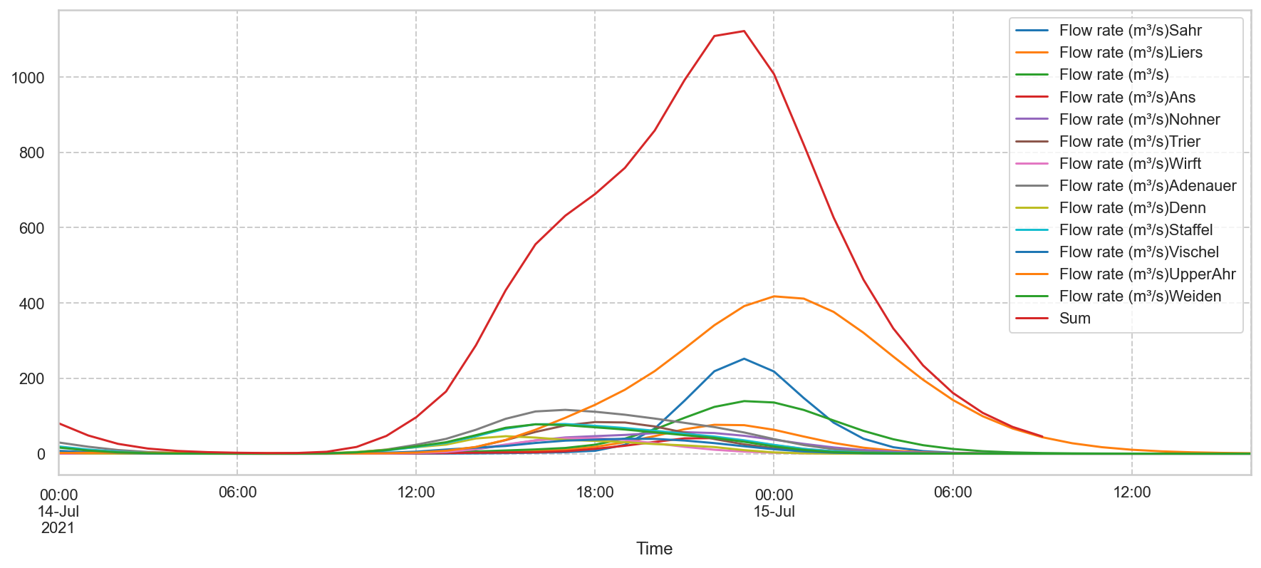
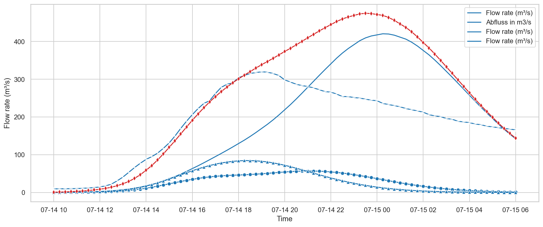
Time lapse of the outflows of tributaries of the Ahr on 14-07-2021

The displayed numbers are the outflows for some principal tributaries, and the combined - and also time-shifted - outflow of them all at Altenahr. $[m³/s]$

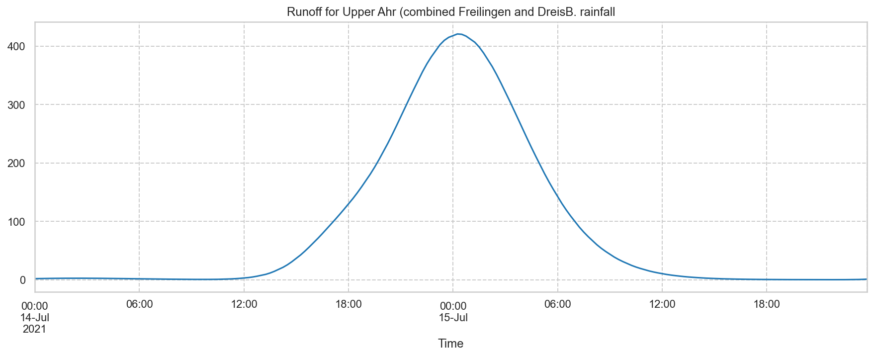
The rainfall peaks in Freilingen and Dreis-Brück occured about 4.5 to 6 hours later than the rainfall peaks on the right bank. This had to do with the very slow movement of the clouds that day (2-2.5km/hr), the orientation of the winds (SSW), and the exceptional amount of rainfall pouring down on the left bank that day.
But I like to mention that the amount of rainfall was +- the same in the morning of 14-07-2021 for all these locations.

Out[48]:
Flow rate (m³/s) Freilingen rain
Time
2021-07-14 10:00:00 85.02 NaN
2021-07-14 11:00:00 71.11 NaN
2021-07-14 12:00:00 63.64 NaN
2021-07-14 13:00:00 66.52 NaN
2021-07-14 14:00:00 84.34 NaN
2021-07-14 15:00:00 122.35 NaN
2021-07-14 16:00:00 184.22 NaN
2021-07-14 17:00:00 269.08 NaN
2021-07-14 18:00:00 370.74 NaN
2021-07-14 19:00:00 479.58 NaN
2021-07-14 20:00:00 585.09 NaN
2021-07-14 21:00:00 677.84 NaN
2021-07-14 22:00:00 750.78 NaN
2021-07-14 23:00:00 799.36 NaN
2021-07-15 00:00:00 821.01 NaN
Out[49]:
Flow rate (m³/s) Freilingen rain Abfluss in m3/s
2021-07-14 00:00:00 71.01 NaN 11.33
2021-07-14 01:00:00 98.23 NaN 12.07
2021-07-14 02:00:00 124.31 NaN 12.07
2021-07-14 03:00:00 144.22 NaN 12.07
2021-07-14 04:00:00 155.11 NaN 12.07
2021-07-14 05:00:00 156.50 NaN 14.00
2021-07-14 06:00:00 149.63 NaN 16.91
2021-07-14 07:00:00 136.69 NaN 21.35
2021-07-14 08:00:00 120.11 NaN 22.73
2021-07-14 09:00:00 102.16 NaN 22.73
2021-07-14 10:00:00 85.02 NaN 22.27
2021-07-14 11:00:00 71.11 NaN 22.27
2021-07-14 12:00:00 63.64 NaN 24.12
2021-07-14 13:00:00 66.52 NaN 30.57
2021-07-14 14:00:00 84.34 NaN 41.12
2021-07-14 15:00:00 122.35 NaN 61.61
2021-07-14 16:00:00 184.22 NaN 87.22
2021-07-14 17:00:00 269.08 NaN 123.43
2021-07-14 18:00:00 370.74 NaN 195.28
2021-07-14 19:00:00 479.58 NaN 309.93
2021-07-14 20:00:00 585.09 NaN NaN
2021-07-14 21:00:00 677.84 NaN NaN
2021-07-14 22:00:00 750.78 NaN NaN
2021-07-14 23:00:00 799.36 NaN NaN

The delay in arrival time is caused by the dynamic aspect of the flood wave: Dynamic wave

  • Amplification
  • Tend to form pulsating flows or surges

The average velocity of each stream should be calculated using manning’s equation u


Flood waves in rivers

The theoretical model for the flood wave used here, is a sudden dam breach. So an immediate height difference, not a gradual one as in river floods.

Source: Course CTB3350, Open Channel Flow, Faculty of Civil Engineering and Geosciences, February 2014, Delft University of Technology

Introduction

Flood waves are in essence humps of water traveling downriver. Stated in more detail, they are temporary increases and decreases of discharge and water level (‘stage’) in a river caused by temporarily enlarged run-off in the catchment area due to heavy rainfall or snow melt, which travel downriver as a wave.
The temporal evolution and dynamics of flood waves differ greatly between the upper reaches and the lower reaches of a river.
In the upper reaches, characterized by relatively steep slopes and a small catchment area, the response to an increased run-off can be quite fast, with rapid variations in flow rate and water level, even to the extent that inhabitants along the river border are taken by surprise, sometimes with fatal consequences.
In contrast, flood waves in the lower river reaches are slow processes, in many cases taking place over several days, due to the larger catchment area, the existence of tributaries, and the greater propagation distance from upstream. Run-off peaks in different part of the larger catchment area do not in general occur simultaneously, so that the maximum of their sum is less than the sum of the individual maxima. Moreover, as we will see, the internal dynamics of the flood wave cause it to flatten and to elongate as it propagates.

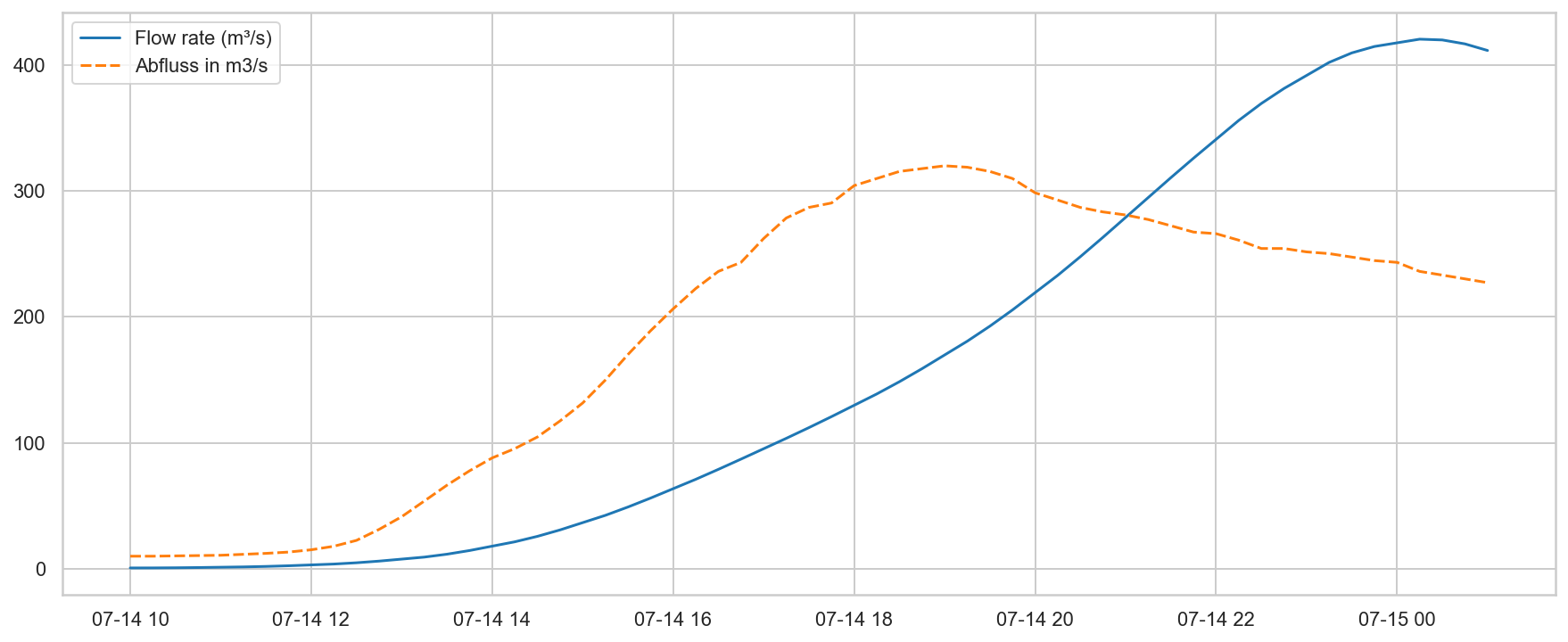
A delay of 1 hour for the combined flow to arrive at Altenahr station, which can be explained by the (clogged) bridges, which were in fact obstacles, is visible.

Out[74]:
Timestamp('2021-07-14 00:00:00')

The high-water wave speed (celerity) is $$c_{hw} = \frac{1}{B}\frac{dQ_u}{d d}= \frac{3}{2}\frac{B_c}{B}U$$

$$σ_s(t) = \sqrt[2]{2 K_0 t} $$

and $i_b$: bed slope, and diffusivity, to be denoted as K: $$K_0 =\frac{Q_0}{2 i_b B}$$

$$𝐾_0= \frac{U_0 d_0}{2 i_b} \frac{B_c}{B}$$
  1. wave speed: $c = \sqrt {gAc/B} =\sqrt {gdB_c/B}$ #m/s
    d= init. depth
  2. discharge: $Q = Bc δh$ #m3/s
    δh: rise in surface elevation
  3. flow velocity: $U = Q/Ac$ # m/s;
    this result also follows from $U = (g/c) δh$ # m/s.
  4. ratio of the advection of momentum relative to the pressure force: $U^2/g δh$ .

Example from the course:

Out[61]:
6.027713773341708
121.5 m²/s
U flow veloc.: 0.24412240782033917 10.849884792015075 0.24412240782033917 m/s
0.040499999999999994 0.0404593951749915

Exercise:

Because of the failure of a dam, a volume of 106 m3 of water is suddenly released in a river, at t = 0 in s = 0, say.
Initially, the flow is uniform; the bed slope is ib = 1.5 × 10⁻⁴, cf = 0.005, d = 3 m, conveyance width Bc = B storage width = 50 m.
Calculate:

  • The value of the diffusivity K (using the initial values of the flow parameters). (Answer: K = 8.9×10^3 m2/s)
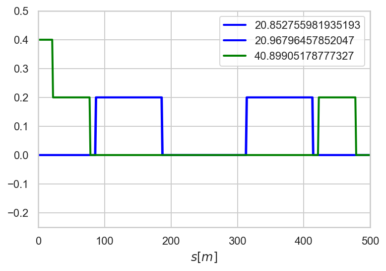
  • The maximum height of the resulting flood wave at t = 5 hrs, and the location smax where this occurs. (Answer: maximum height is 0.45 m, smax= 25 km)
  • Explain why the maximum height of question (b) is less than the maximum height occurring in s = smax during the passage of the flood wave, and verify this with calculations for a few chosen instants near the time t = 5 hrs.
Out[36]:
5.424942396007538
Out[20]:
0.767
Out[22]:
13809.648800747977
length: 0.7066666666666667 0.00015000000000000001
K_0 7066.666666666666
t 18000.0 σ_s 17899.720668211557
Out[25]:
0.7159888267284623

recorded outflow at Müsch

K_0 496.1240310077519
Out[66]:
6.484

Lets take the diffusion of the peak at Musch to Altenahr... which is probably too distorted to be detectable, by the presence of wave narrowing and blocking bridges.

t 3888.8888888888887 σ_s 1964.368209728926
Out[68]:
1.08025

$σ_s$ increases in time proportional to √t: the wave elongates.

62.36095644623236 31.18047822311618 s

For the wave at t1 and t2 the ratio V/B [length/width] remains constant.

So I need to get the water level and base differences for Musch and other tributaries, and compare them with these at Altenahr: that's too much hussle and too many unknowns.

Out[129]:
13108.61423

Influence of variable free-surface slope

In the preceding section, the variations in the slope of the free surface, which accompany the passage of a flood wave, were ignored. Actually, the slope varies, being larger than the slope in uniform flow (ib) in the leading part of a flood wave, i.e. at rising river stage in a fixed point, whereas it is less than ib in the trailing part, i.e. at falling river stage. Therefore, at a given stage, the discharge is greater when the surface elevation rises than when it falls.
This is a manifestation of the phenomenon of hysteresis.

Out[85]:
Flow rate (m³/s)
Time
2021-07-13 00:00:00 0.00e+00
2021-07-13 00:15:00 0.00e+00
2021-07-13 00:30:00 0.00e+00
2021-07-13 00:45:00 1.33e-06
2021-07-13 01:00:00 4.72e-06
... ...
2021-07-17 07:30:00 0.00e+00
2021-07-17 07:45:00 0.00e+00
2021-07-17 08:00:00 0.00e+00
2021-07-17 08:15:00 0.00e+00
2021-07-17 08:30:00 0.00e+00

419 rows × 1 columns

Out[77]:
Wasserstand in cm
Datum
27.06.2021 18:00 35.0
27.06.2021 18:15 35.0
27.06.2021 18:30 35.0
27.06.2021 18:45 35.0
27.06.2021 19:00 35.0
... ...
15.07.2021 22:45 NaN
15.07.2021 23:00 NaN
15.07.2021 23:15 NaN
15.07.2021 23:30 NaN
15.07.2021 23:45 NaN

1752 rows × 1 columns

Out[78]:
Wasserstand in cm
Datum
2021-06-27 18:00:00 35.0
2021-06-27 18:15:00 35.0
2021-06-27 18:30:00 35.0
2021-06-27 18:45:00 35.0
2021-06-27 19:00:00 35.0
... ...
2021-07-15 22:45:00 NaN
2021-07-15 23:00:00 NaN
2021-07-15 23:15:00 NaN
2021-07-15 23:30:00 NaN
2021-07-15 23:45:00 NaN

1752 rows × 1 columns

Out[75]:
Wasserstand in cm Abfluss in m3/s
Datum
2021-07-12 00:00:00 71.0 6.25
2021-07-12 00:15:00 71.0 6.25
2021-07-12 00:30:00 71.0 6.25
2021-07-12 00:45:00 71.0 6.25
2021-07-12 01:00:00 71.0 6.25
... ... ...
2021-07-14 22:45:00 NaN NaN
2021-07-14 23:00:00 NaN NaN
2021-07-14 23:15:00 NaN NaN
2021-07-14 23:30:00 NaN NaN
2021-07-14 23:45:00 NaN NaN

288 rows × 2 columns

Out[87]:
Wasserstand in cm Flow rate (m³/s)
2021-07-13 00:00:00 45.0 0.00e+00
2021-07-13 00:15:00 45.0 0.00e+00
2021-07-13 00:30:00 45.0 0.00e+00
2021-07-13 00:45:00 46.0 1.33e-06
2021-07-13 01:00:00 46.0 4.72e-06
... ... ...
2021-07-15 22:45:00 NaN 2.08e+00
2021-07-15 23:00:00 NaN 1.91e+00
2021-07-15 23:15:00 NaN 1.74e+00
2021-07-15 23:30:00 NaN 1.56e+00
2021-07-15 23:45:00 NaN 1.40e+00

288 rows × 2 columns

The phenomenon of hysteresis in Musch and Altenahr.

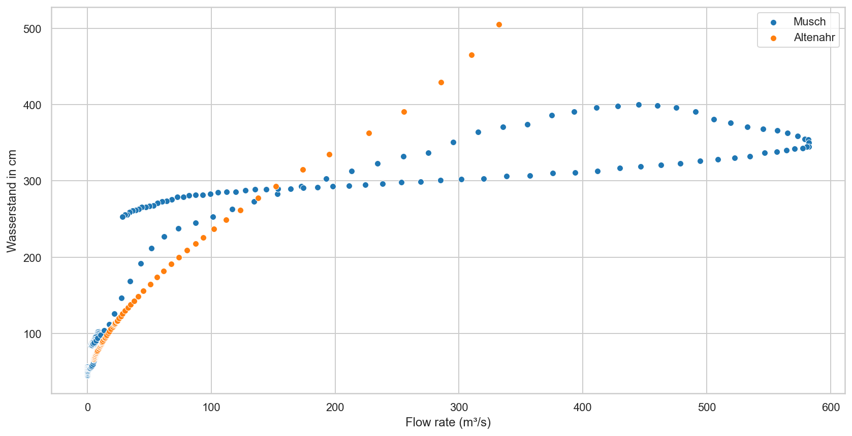
From the plot we can conclude: the peak debit at Müsch happened 3:00-3:30 hours before the peak water level.
Also the orange curve is very steep, which points out that the water mass cannot pass swiftly through the narrow valley.

First I thought I'd need to differentiate...

elementary-wave.py