Groundwater flow – Solving PDEs using ODE solvers¶

Source: incomplete course notes for MatLab solvers, Session 4.2, from the NNESMO website:
https://nnesmo2019.webspace.durham.ac.uk/practicals/session42/
Dr Simon A Mathias, Department of Earth Sciences, Durham University

Contents¶

• Groundwater flow in a confined aquifer
• Spatial discretisation using finite differences
• Development of the solution code
• Plotting the results and comparing to an analytical solution
• Stiff and non-stiff problems
• Specifying the Jacobian pattern

Groundwater flow in a confined aquifer¶

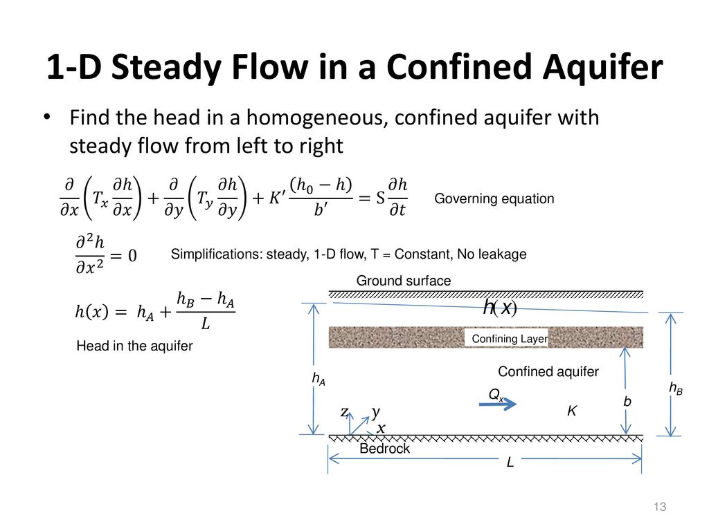
A confined aquifer is bounded to the West by a lake and to the East by an impermeable fault zone.
The aquifer is homogenous and isotropic and characterised by a transmissivity of 800 and a storativity of 0.01.
The edge of the lake lies parallel to the fault zone and is separated by a distance of 1600 m.
Initially the lake level is 50 m AOD (metres above ordinance datum).
After a significant episode of snow melt in the mountains above, the water level in the lake is suddenly raised to 53 m AOD.

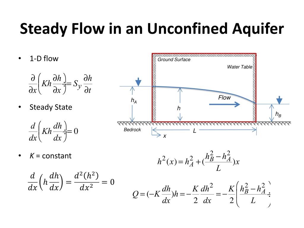
The governing equation for one dimensional groundwater flow in a (un)confined aquifer takes the form

$\frac {d}{dx} K \frac {dh}{dx} = S \frac {dh}{dt}$

where S [-] is the aquifer storativity (which relates to the bulk compressibility of the aquifer),
h [L] is the hydraulic head, t [T] is time, L [L] is distance and
Q is $q*h$ [m^2/s] is the volumetric flow rate per unit breadth of confined aquifer, found from

where T is the transmissivity of the aquifer (which relates to the bulk permeability of the aquifer).

Discharge per unit width of aquifer = $({Piezometric_{Head}}_{Upstream}-{Piezometric_{Head}}_{DownstreamEnd})/Length*{Coefficient}_{permeability}*{Aquifer}_{Thickness}$
$$q=\frac{(h_o-h_1)}{L}\cdot k \cdot b$$

The relevant initial and boundary conditions can be written as follows:

$t_0$= 0
$t_x$= 0.1, 0.3, 0.5, 1, 3, 5 in days
T= 800
S= 0.01
L= 1600
$h_I$= $h_1$= 50
$h_0$= 53
$$T dy^2/dx^2 - 0 dy/dx =S u$$ and $$u= dt$$

Volume of Confined Water for a change in head = $SAΔh$ where:

• Volume = volume drained from a confined aquifer for a hydraulic head change, Δh, over an area, A (L³)

• S = storativity (dimensionless)

• A = area over which the head change occurs (L²)

• Δh = change in head (L)

• Discharge per unit width of aquifer - (Measured in M³ per Second)

  • Discharge per unit width of aquifer is the rate of total discharge in the channel to the width considered.

• Transmissivity - (Measured in M² per Second)

  • Transmissivity is the rate at which groundwater flows horizontally through an aquifer

Use the solver 'odeint' to develop a one-dimensional finite difference model to estimate the hydraulic head within the aquifer.

Show the results as a plot of hydraulic head against distance, for the following times: 0.1, 0.3, 0.5, 1, 3, 5 and 7 days.

Spatial discretisation using finite differences¶

The above problem is an example of a partial differential equation (PDE). However, if we discretise the problem in space, the problem becomes a coupled set of ordinary differential equations (ODE) with respect to time. Here we will use odeint to solve the large set of coupled ODEs that results from the spatial discretisation. We will use finite difference for spatial discretisation. However, other methods such as finite elements and pseudospectral methods can also be used in a similar way.

Let us consider a set of discrete points on the x-axis: $x_n$.

The corresponding set of hydraulic heads can be written as: h(x).

An approximation of flow per unit breadth, $q^*$, can be found from $q_x =-k_x dh/dx$

but note that these flow rates are defined at an alternative set of points: $x_b$.

The resulting set of ODEs to be solved takes the form $d/dx K dh/dx = S \cdot dh/dt$

Letting ∆x → 0 and ∆t → 0 in (5) leads to the one-dimensional groundwater flow equation, $∂h^2/∂x^2=1/k(∂h/∂t)−R(x,t)/K$
R=recharge, for 0<x<a, t>0, (6) where we have introduced the hydraulic diffusivity k via $k=K/S_s$.

Recall that the relationship between and is $T = K b$

Furthermore it can be shown that

$h_2=53 m$
$c_1= \frac {(h_2^2-h_1^2)}{L}+(N \cdot L/K)$
$c_2= h_1^2$
$h^2(x)=+h_1^2- (h_2^2-h_1^2)\frac {x}{L}+ \frac {Nx}{K} (L-x)$

Development of the solution code¶

Create a new script-file:

function onedimex()¶

1. Solves the one-dimensional confined aquifer flow equation using the python ODE solver 'odeint', when using the function argument 'odeint'.

This older solver has some perks:

• Solves a system of ordinary differential equations using lsoda from the FORTRAN library odepack.
• Solves the initial value problem for both stiff and non-stiff systems of first order ode's.

2. otherwise this function solves the one-dimensional confined aquifer flow equation using the python ODE solver 'solve_ivp' .

So far all we have done is written some comments explaining what some of the subsequent variables are and defined the model parameter values.

The next step is to determine the locations on the x-axis that we are going to solve for.

In the above variable list we have x and xB. It is planned that x and xB will be vectors containing and , respectively.

Another point to note is that $x_B(1)=0$ and $x_B{(N+1)}=L$.

Add the following code to provide a discretisation for 20 equally spaced solution points

Next we will add some code to define the times of interest and a vector containing the initial values for .

solve_ivp¶

This is the solver which should be used for new code, according to scipy. We need to use solver/method 'LSODA', instead of the default 'RK45' for handling possible stiffness.

stand alone code for solver_ivp()¶

so the new solver can use the finite diff. method.

Of course we need to write the ODE function as well.

function MYodefun¶

This function calculates derivatives and contains also a function for the analytical solution.

Analytical solution¶

3D surface subplots¶

meshgrid test¶

Most of the above code in the ODE function is self-explanatory. However, pay close attention to how the boundary conditions are applied.

The fixed head boundary, associated with the lake, is applied by concatenating the boundary head, h0, and its associated location, xB(1), to the h and x vectors, respectively, prior to finding the derivatives, .

The zero flux boundary, associated with the fault zone, is applied by simply concatenating a zero to the Q vector.

Plotting the results and comparing to an analytical solution¶

Whenever developing numerical models it is always important to study your results and try to compare these to analytical solutions where possible.

The problem being solved here has an analytical solution for the special case where . Our finite difference model should produce very similar results to the analytical solution until the pressure wave hits the bounday at .

The analytical solution takes the form

Add the following subfunction to your script-file, which contains an implementation of the analytical solution.

Animation of hydraulic heads over time¶

DataFrame composition¶

Step changes in surface water level: Edelman formula's¶

basic plot head and Qx vs x¶

basic plot head and Qx vs time¶

Stiff and non-stiff problems¶

At the moment, we are solving the diffusion problem using a uniform space-step. Just as we can benefit from having time-step refinement during periods of high activity, we can also benefit from spatial grid refinement in areas of high activity.

In this particular case, most of the activity is occurring around where the fixed head boundary exists. Therefore a more appropriate spatial discretisation is arguably achieved using the code:

$x_B=[0,np.logspace(-3,0,N)*L]$

which logarithmically spaces the finite different points over three orders of magnitude, with the smallest grid spacing around $h(53)$.

Add the above code for $x_B$ to the existing code and run.

You will find the solution takes forever to complete. The reason is that the simulation has become very stiff. Type "ctrl c" in the command window to terminate the simulation.

Sets of coupled ODEs are said to be stiff when the ODEs move at very different rates. By refining the spatial grid, we have created a system whereby the ODEs near are very fast whilst the ODEs near are very slow.

The ode45 solver is not good for stiff problems. Instead, try and use the solver ode15s by changing the code to say

You can read more about how ode15s works in the help files.

Specifying the Jacobian pattern¶

For large sets of ODEs, the stiff solvers are much more efficient if you specify the Jacobian pattern a priori. So what is the Jacobian pattern?

For the example under consideration, let us define

Now consider the vectors and .

Therefore, the Jacobian pattern for this problem can be seen to be a tri-diagonal sparse matrix of the form:

To implement this Jacobian pattern within your code, replace the line

S = spdiags(Bin,d,m,n) creates an m-by-n sparse matrix S by taking the columns of Bin and placing them along the diagonals specified by d. spdiags(data, diags, m, n, format)