Table of Contents

• 1  Italian waterbodies data: water source Lupa
  • 1.1  Data set description
    • 1.1.1  Aquifer
    • 1.1.2  Water spring
    • 1.1.3  River Arno
    • 1.1.4  Lake Bilancino
  • 1.2  Introduction
  • 1.3  Methodology
• 2  Water spring Lupa
  • • 2.0.1  References
    • 2.0.2  Evolution of the outflow over the last 11 years
  • 2.1  taking the differences
    • 2.1.1  logarithms of the flow rate.
    • 2.1.2  pmdArima: introduction
      • 2.1.2.1  2020
  • 2.2  Rainfall
    • 2.2.1  Annual Water Budget Ratio (AWBR)
  • 2.3  Arrone rainfall addition
    • 2.3.1  Ancaiano daily pluviometry
      • 2.3.1.1  Ancaiano pluviometry 2009 and 2020-2022
    • 2.3.2  SPI
      • 2.3.2.1  SPI 12 calculation via module standard-precip
      • 2.3.2.2  SPEI
    • 2.3.3  Soil moisture condition
    • 2.3.4  TR-55: 'Urban Hydrology for Small Watersheds'
    • 2.3.5  SCS CN- or curve number method
      • 2.3.5.1  Runoff Equation
      • 2.3.5.2  SCS Hydrologic Soil Groups: Soil textures
    • 2.3.6  Runoff curve numbers for cultivated/other agricultural lands and soil types
    • 2.3.7  Curve-number map for Umbria Region
    • 2.3.8  Calculate runoff depth
    • 2.3.9  The determination of CN values: by formula method, or by conversion table method
  • 2.4  Infiltration coefficients method
    • 2.4.1  Calculate the infiltrate amount i.f.o mm/day rainfall
  • 2.5  Temperature
    • 2.5.1  Heat index per year
    • 2.5.2  T2M_MAX, T2M_MIN, relative humidity
    • 2.5.3  AET/PET - Drought Index
  • 2.6  Flow rate original data
    • 2.6.1  Rolling sums monthly
    • 2.6.2  The variability index (Meinzer, 1927)
    • 2.6.3  First attempt to gather better flow rate data...
    • 2.6.4  resample flow rate 2010-2019 monthly
    • 2.6.5  The 2012 series
    • 2.6.6  Maximum 1999-2011, Minimum 1999-2011, Mean 1999-2011
    • 2.6.7  Mean of period 2010-2020 vs. the Mean of 1999-2011
      • 2.6.7.1  Set list of distributions to test
    • 2.6.8  Conversion of units etc...
    • 2.6.9  Yearly and monthly aggregates
      • 2.6.9.1  statsmodels api
      • 2.6.9.2  Netto infiltration - outflow
    • 2.6.10  statsmodels SARIMAX
  • 2.7  pmdArima examples
    • 2.7.1  Fitting an auto_arima model
    • 2.7.2  Displaying key timeseries statistics
    • 2.7.3  Array differencing
    • 2.7.4  Modeling quasi-seasonal trends with date features
    • 2.7.5  Rolling sums in m³
      • 2.7.5.1  Rainfall rolling sums
      • 2.7.5.2  Cumulative sums for the rainfall and outflow in cubic meters.
      • 2.7.5.3  Water balance m³ rainfall - water spring outflow
    • 2.7.6  Cross-correlation and Auto-correlation
      • 2.7.6.1  Cross-correlation daily and weekly data
      • 2.7.6.2  Cross-correlation daily and weekly data
    • 2.7.7  Recession coefficient or coefficient of depletion
    • 2.7.8  Plots of absolute vs. mean values of Q / t
    • 2.7.9  Outflow of 2017
    • 2.7.10  Calculating evapotranspiration method 1
    • 2.7.11  Calculating evapotranspiration method 2
    • 2.7.12  Evapotranspiration water spring Peschiera
  • 2.8  Solar Radiation
    • 2.8.1  Hargreaves method
      • 2.8.1.1  Simplification through the relation T_avg - T_max - T_min
      • 2.8.1.2  W/m² to MJ/m²
      • 2.8.1.3  extract T_max - T_min for Hargreaves formula method
  • 2.9  Random forest regression with XGBoost
    • 2.9.1  based on poor data
    • 2.9.2  Predictions based on much better data
    • 2.9.3  We try the 'best' dataset here
    • 2.9.4  We try the 'best' dataset here [2]: TimeSeriesSplit
  • 2.10  Prediction of flow rate of the source
    • 2.10.1  Random Forest Regressor (sklearn)
      • 2.10.1.1  Permutation Feature Importance
      • 2.10.1.2  RF regressor metrics
      • 2.10.1.3  RF regressor predictions vs. observations
      • 2.10.1.4  Predictionplot: Lupa source flow rate
      • 2.10.1.5  Method 2 to compare results
      • 2.10.1.6  Time-related feature engineering: Trigonometric_features
    • 2.10.2  ExtraTreesRegressor
      • 2.10.2.1  ET regressor metrics
      • 2.10.2.2  ET regressor: predictions vs. observations
      • 2.10.2.3  Predictionplot: observed vs. estimated source flow rate
  • 2.11  Revisiting the Lupa data
    • • 2.11.0.1  2009 and 2020-2022 debit data
    • 2.11.1  Calculation of the recession coefficients α over a span of several days.
    • 2.11.2  determination of Correlation coefficients rain-outflow
      • 2.11.2.1  Rainfall_Terni vs infiltrate comparison
      • 2.11.2.2  Outflow data of 2009 and 2020-2021:
      • 2.11.2.3  Correlations: monthly shifted
  • 2.12  Alternative approach of considering P5 in the SCS-CN model
  • 2.13  The older and more recent water spring parameters in overview table.
    • • 2.13.0.1  The slope of the recession curve vs. maximum outflow

Italian waterbodies data: water source Lupa

Can you help preserve "blue gold" using data to predict water availability?
Acea Smart Water Analytics

https://www.kaggle.com/c/acea-water-prediction/data

Data set description

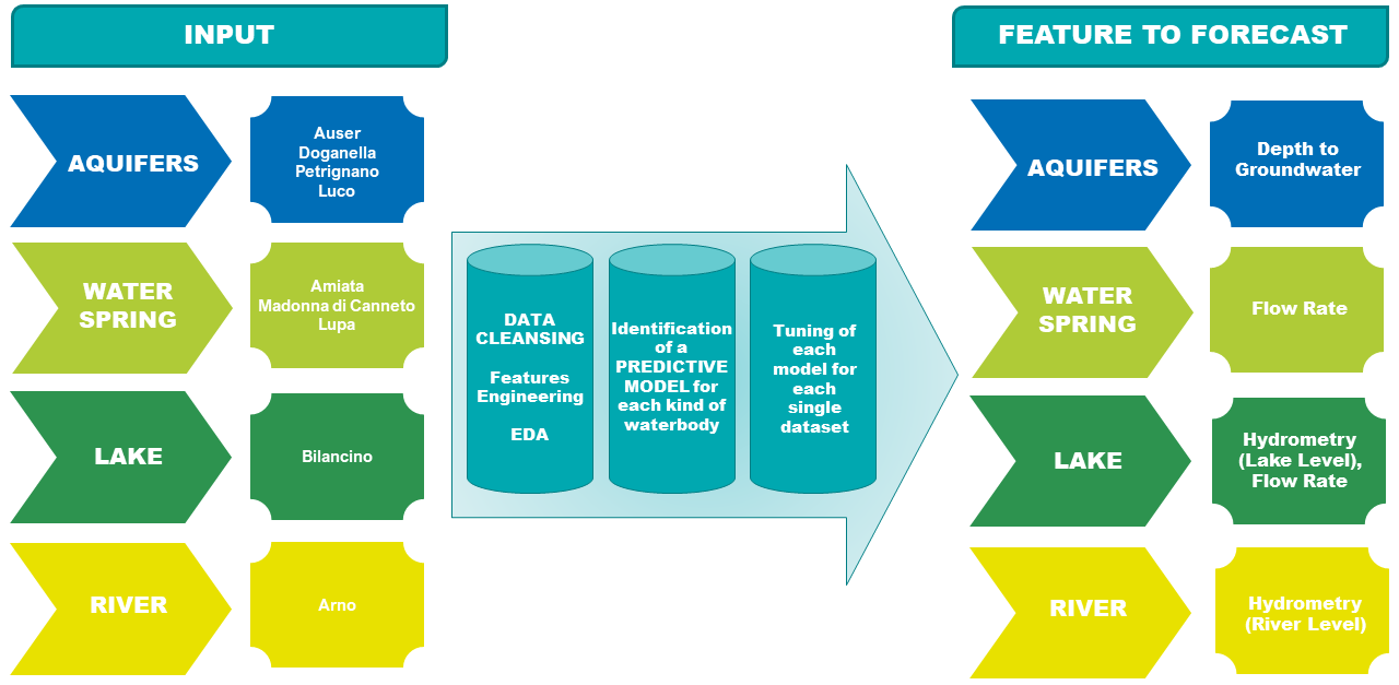
This competition uses nine different datasets, completely independent and not linked to each other. Each dataset can represent a different kind of waterbody. As each waterbody is different from the other, the related features as well are different from each other. So, if for instance we consider a water spring we notice that its features are different from the lake’s one. This is correct and reflects the behavior and characteristics of each waterbody. The Acea Group deals with four different type of waterbodies: water spring (for which three datasets are provided), lake (for which a dataset is provided), river (for which a dataset is provided) and aquifers (for which four datasets are provided).

Let’s see how these nine waterbodies differ from each other.

Aquifer

Auser

• This waterbody consists of two subsystems, called NORTH and SOUTH, where the former partly influences the behavior of the latter. Indeed, the north subsystem is a water table (or unconfined) aquifer while the south subsystem is an artesian (or confined) groundwater. The levels of the NORTH sector are represented by the values of the SAL, PAG, CoS and DIEC wells, while the levels of the SOUTH sector by the LT2 well.

Petrignano Aquifer

• The wells field of the alluvial plain between Ospedalicchio di Bastia Umbra and Petrignano is fed by three underground aquifers separated by low permeability septa. The aquifer can be considered a water table groundwater and is also fed by the Chiascio river. The groundwater levels are influenced by the following parameters: rainfall, depth to groundwater, temperatures and drainage volumes, level of the Chiascio river.

Doganella Aquifer

• The wells field Doganella is fed by two underground aquifers not fed by rivers or lakes but fed by meteoric infiltration. The upper aquifer is a water table with a thickness of about 30m. The lower aquifer is a semi-confined artesian aquifer with a thickness of 50m and is located inside lavas and tufa products. These aquifers are accessed through wells called Well 1, ..., Well 9. Approximately 80 \% of the drainage volumes come from the artesian aquifer. The aquifer levels are influenced by the following parameters: rainfall, humidity, subsoil, temperatures and drainage volumes.

Luco Aquifer

• The Luco wells field is fed by an underground aquifer. This aquifer not fed by rivers or lakes but by meteoric infiltration at the extremes of the impermeable sedimentary layers. Such aquifer is accessed through wells called Well 1, Well 3 and Well 4 and is influenced by the following parameters: rainfall, depth to groundwater, temperature and drainage volumes.

Water spring

Amiata

• The Amiata waterbody is composed of a volcanic aquifer not fed by rivers or lakes but fed by meteoric infiltration. This aquifer is accessed through Ermicciolo, Arbure, Bugnano and Galleria Alta water springs. The levels and volumes of the four sources are influenced by the parameters: rainfall, depth to groundwater, hydrometry, temperatures and drainage volumes.

Madonna di Canneto

• The Madonna di Canneto spring is situated at an altitude of 1010m above sea level in the Canneto valley. It does not consist of an aquifer and its source is supplied by the water catchment area of the river Melfa.
• Settefrati is a commune with an altitude of 784 m and surface area of 50,6 km².

Lupa

• This water spring is located in the Rosciano Valley, on the left side of the Nera river. The waters emerge at an altitude of about 375 meters above sea level through a long draining tunnel that crosses, in its final section, lithotypes and essentially calcareous rocks. It provides drinking water to the city of Terni and the towns around it.

River Arno

• Arno is the second largest river in peninsular Italy and the main waterway in Tuscany and it has a relatively torrential regime, due to the nature of the surrounding soils (marl and impermeable clays). Arno results to be the main source of water supply of the metropolitan area of Florence-Prato-Pistoia. The availability of water for this waterbody is evaluated by checking the hydrometric level of the river at the section of Nave di Rosano.

Lake Bilancino

• Bilancino lake is an artificial lake located in the municipality of Barberino di Mugello (about 50 km from Florence). It is used to refill the Arno river during the summer months. Indeed, during the winter months, the lake is filled up and then, during the summer months, the water of the lake is poured into the Arno river.

Each waterbody has its own different features to be predicted. The table below shows the expected feature to forecast for each waterbody.

It is of the utmost importance to notice that some features like rainfall and temperature, which are present in each dataset, don’t go alongside the date. Indeed, both rainfall and temperature affect features like level, flow, depth to groundwater and hydrometry some time after it fell down. This means, for instance, that rain fell on 1st January doesn’t affect the mentioned features right the same day but some time later. As we don’t know how many days/weeks/months later rainfall affects these features, this is another aspect to keep into consideration when analyzing the dataset.

A short, tabular description of the waterbodies is available also downloading all datasets.

More information about the behavior of each kind of waterbody can be found at the following links:

• Aquifer https://en.wikipedia.org/wiki/Aquifer
• Water spring https://en.wikipedia.org/wiki/Spring_(hydrology)
• River https://en.wikipedia.org/wiki/River
• Lake https://en.wikipedia.org/wiki/Lake

C:\Users\VanOp\AppData\Local\Temp\ipykernel_15916\1212899292.py:14: DeprecationWarning: Importing display from IPython.core.display is deprecated since IPython 7.14, please import from IPython display
  from IPython.core.display import display, HTML, SVG

Autosaving every 500 seconds

---

'%.4f'

Introduction

In recent years, long and frequent droughts have affected many countries in the world. These events require an ever more careful and rational management of water resources. Most of the globe’s unfrozen freshwater reserves are stored in aquifers. Groundwater is generally a renewable resource that shows good quality and resilience to fluctuations. Thus, if properly managed, groundwater could ensure long-term supply in order to meet increasing water demand.

For this purpose, it is of crucial importance to be able to predict the flow rates provided by springs. These represent the transitions from groundwater to surface water and reflect the dynamics of the aquifer, with the whole flow system behind. Moreover, spring influences water bodies into which they discharge. The importance of springs in groundwater research is highlighted in some significant contributions. In-depth studies on springs started only after the concept of sustainability was introduced in the management of water resources.

A spring hydrograph is the consequence of several processes governing the transformation of precipitation in the spring recharge area into the single output discharge at the spring. A water balance states that the change rate in water stored in the feeding aquifer is balanced by the rate at which water flows into and out of the aquifer. A quantitative water balance generally has to take the following terms into account: precipitation, infiltration, surface runoff, evapotranspiration, groundwater recharge, soil moisture deficit, spring discharge, lateral inflow to the aquifer, leakage between the aquifer and the underlying aquitard, well pumpage from the aquifer, and change of the storage in the aquifer.

In many cases, the evaluation of the terms of the water balance is very complicated. The complexity of the problem arises from many factors: hydrologic, hydrographic, and hydrogeological features, geologic and geomorphologic characteristics, land use, land cover, water withdrawals, and climatic conditions.

Even more complicated would be to estimate future spring discharges by using a model based on the balance equations. Therefore, simplified approaches are frequently pursued for practical purposes.

Many authors have addressed the problem of correlating the spring discharges to the rainfall through different approaches...

Methodology

The Methodology to use depends on the properties of the water source, local geology, and the unknown parameters. There is no clear cut path.
An example of a methodology is presented in the next illustration. It provides a view how the topics I handled are related to each other, and how unknown info and truthfull data matters to obtain a reasonable result.

Water spring Lupa

<!img src="http://vanoproy.be/css/Lupa.jpg"-->

432000 l/h 10368000 l/d

Nella dorsale montuosa che occupa la parte orientale della regione, esistono due sistemi idrogeologici separati dalla linea tettonica denominata “linea della Valnerina”, dove è individuabile un limite di permeabilità che corre a quote variabili tra 350 e 700 m s.l.m.: a sud il “Sistema della Valnerina” e a nord il “Sistema dell’Umbria nord-orientale”.
Con “Sistema della Valnerina”, viene identificata l’imponente struttura idrogeologica presente al margine sud-orientale del territorio regionale. Questa si estende dal corso del Fiume Nera, ad ovest, fino alla linea tettonica Ancona-Anzio, la sua superficie in territorio umbro è di circa 1.100 km2. Il sistema nel suo complesso è caratterizzato dalla presenza di una serie di acquiferi costituiti principalmente dalle formazioni della Scaglia s.l., della Maiolica e della Corniola-Calcare Massiccio. Questi presentano comunque continuità idraulica sia per contatti laterali che verticali. La formazione della Scaglia s.l. ospita l’acquifero più superficiale, che dà luogo a sorgenti puntuali per lo più di modesta portata e contribuisce all’alimentazione del deflusso di base dei corsi d’acqua o alla ricarica degli acquiferi più profondi.
I livelli piezometrici raggiungono quote superiori a 800 m s.l.m. e decrescono da est ad ovest fino a raggiungere la minima quota in corrispondenza dell'alveo del Nera, che costituisce il livello di base principale del sistema. Lungo questa linea di drenaggio dominante, diretta SO-NE, si hanno importanti sorgenti lineari responsabili di notevoli incrementi di portata del fiume Nera. Studi pregressi hanno stimato che, lungo il tratto umbro del fiume Nera, si hanno emergenze in alveo per una portata media complessiva superiore a 15 m3 al secondo. Oltre alle emergenze in alveo, si trovano numerose sorgenti localizzate, che rilasciano una frazione molto più modesta delle acque della struttura, valutabile in qualche centinaio di litri al secondo. Le restituzioni sorgentizie, di tipo sia lineare sia puntuale, sono stimate in un volume di circa 700 Mm3 annui.

The Lupa water spring is located in the central Apennines range on the left side of the river Nera near Arenno, and has an historical flowrate of about 120 l/sec. The aquifer of this karstic system contains deposits named Scaglia. The net recharge of the "Scaglia Calcarea" complex proved to be 170-425 mm/year.
The hydrological unit is called "Monte Coscerno", which has an infiltration efficiency estimated at 475 mm per year based on data from 1997-2007.
Monte Coscerno feeds several waterbodies: the river Nera, the stream F. di Castellone, and 3 notable continuous water springs. The infiltration efficiency increases going from North to South.

Spring	Elevation	Outflow (l/s)
Scheggino	300	200
Lupa	365	125
Pacce	475	80
Castellone	450-325	115

The combined outflow of all the waterbodies of the Monte Coscerno system is +-:

3615 Lupa: 3.46 %, estimated drainage area: 8.3333

520 Lupa: 24 %

Update on estimated drainage area:

• a study from 1996 estimates Lupa's drainage area 10-12 km².
• however it was not mentioned if this value relates to the short term, middle or long term "outflow component" related to 3 waterbearing layers. But I assume it would be short term, which is the most responsive layer.

Location 42.5800 N 12.8132 E
Soils of Italy

References

• Linee Guida sugli Indicatori di Siccità e Scarsità Idrica da utilizzare nelle attività degli Osservatori Permanenti per gli Utilizzi Idrici - Stato Attuale e Prospettive Future (in...), Stefano Mariani, Emanuele Romano,Italian National Research, Giovanni Braca,Barbara Lastoria, Institute for Environmental Protection and Research. Technical Report · June 2018
• SPRINGS (Classification, function,capturing), Soulios G., Dep. of Geology, Aristotle University of Thessaloniki, Bulletin of the Geological Society of Greece, Vol. 43, (2010), DOI: 10.12681/bgsg.11174
• Urban hydrology for small watersheds. Tech. Release 55., U.S. Department of Agriculture, Soil Conservation Service. 1986.
• RUNOFF CURVE NUMBER METHOD: Examination of the Initial Abstraction Ratio, Richard H. Hawkins, Professor, University of Arizona, Tucson, (USDA, Natural Resources Conservation Service, 2002)
• Chapter 20 - Watershed Yield, Part 630 Hydrology, National Engineering Handbook, 2009, USDA
• Groundwater - Hydrology of springs, Chapter 4 - Spring discharge hydrograph, Neven Kresic, Amec Foster Wheeler, Bonacci o., Univ Split Croatia, (2010)
• Karst Groundwater Availability and Sustainable Development, F. Fiorillo, V. Ristić Vakanjac, I. Jemcov, S. P Milanovic, University of Belgrade, February 2015), DOI: 10.1007/978-3-319-12850-4_15
• Predicted Maps for Soil Organic Matter Evaluation: The Case of Abruzzo Region (Italy). Piccini, C.; Francaviglia, R.; Marchetti, A., Land 2020, 9, 349. https://doi.org/10.3390/land9100349
• Machine Learning Models for Spring Discharge Forecasting, Francesco Granata , Michele Saroli, Giovanni de Marinis, and Rudy Gargano, 2018, https://doi.org/10.1155/2018/8328167
• Comparison of antecedent precipitation based rainfall-runoff models, Pankaj Upreti; C. S. P. Ojha, Water Supply (2021) 21 (5): 2122–2138.
• Effective infiltration variability in the Umbria-Marche carbonate aquifers of central Italy, Lucia Mastrorillo, Marco Petitta - Journal of Mediterranean Earth Sciences 2 (2010), 9-18, doi:10.3304/JMES.2010.002

• Water Balance and Soil Moisture Deficit of Different Vegetation Units under Semiarid Conditions in the Andes of Southern Ecuador - Andreas Fries, Karen Silva, Franz Pucha-Cofrep, Fernando Oñate-Valdivieso and Pablo Ochoa-Cueva; Climate 2020, 8(2), 30; https://doi.org/10.3390/cli8020030

• The "APEX" Agricultural Policy Environmental eXtender Model theoretical documentation, Version 0604, BREC Report # 2008-17.

• Fraction of Absorbed Photosynthetically Active Radiation https://land.copernicus.eu/global/products/fapar

	Date	Rainfall_Terni	Flow_Rate_Lupa
0	01/01/2009	2.8	NaN
1	02/01/2009	2.8	NaN
2	03/01/2009	2.8	NaN
3	04/01/2009	2.8	NaN
4	05/01/2009	2.8	NaN

I started with the original dataset of ACEA, which only had errorprone flowrate data for uncomplete 3 years. So I felt I was forced to find better data, which I found on some Italian websites. Later I'd merge the original with the missing flow rate data. But after completing that, the monthly rainfall data was no longer good enough. Moreover this was Terni pluvio data, which is 11 km away from Lupa, plus it is located on the wrong side of the waterbody.
In short: I collected new meaningfull data, and gradually created a new data set

	Date	Rainfall_Terni	Flow_Rate_Lupa	doy	Month	Year	ET01	Infilt_	Infiltsum	Rainfall_Ter	Flow_Rate_Lup	Infilt_m3
0	2009-01-01	2.8	135.47	1.0	1.0	2009.0	NaN	NaN	NaN	352422.0	11704.61	NaN
1	2009-01-02	2.8	135.24	2.0	1.0	2009.0	NaN	NaN	NaN	352422.0	11684.74	NaN
2	2009-01-03	2.8	135.17	3.0	1.0	2009.0	NaN	NaN	NaN	352422.0	11678.69	NaN
3	2009-01-04	2.8	134.87	4.0	1.0	2009.0	NaN	NaN	NaN	352422.0	11652.77	NaN
4	2009-01-05	2.8	134.80	5.0	1.0	2009.0	NaN	NaN	NaN	352422.0	11646.72	NaN

	Date	Rainfall_Terni	Flow_Rate_Lupa	doy	Month	Year	ET01	Infilt_	Infiltsum	Rainfall_Ter	Flow_Rate_Lup	Infilt_m3	Week
0	2010-01-01	3.27	82.24	1.0	1.0	2010.0	1.34	1.93	1.93	412398.0	7105.54	143639.37	53
1	2010-01-02	3.27	88.90	2.0	1.0	2010.0	1.70	1.57	3.51	412398.0	7680.96	130966.87	53
2	2010-01-03	3.27	93.56	3.0	1.0	2010.0	0.94	2.33	5.84	412398.0	8083.58	157582.00	53
3	2010-01-04	3.27	96.63	4.0	1.0	2010.0	1.00	2.28	8.12	412398.0	8348.83	155554.40	1
4	2010-01-05	3.27	98.65	5.0	1.0	2010.0	1.28	1.99	10.11	412398.0	8523.36	145736.74	1

	Rainfall_Terni	Flow_Rate_Lupa	doy	Month	Year	ET01
Date
2010-01-01	3.27	82.24	1	1	2010	1.34
2010-01-02	3.27	88.90	2	1	2010	1.70
2010-01-03	3.27	93.56	3	1	2010	0.94
2010-01-04	3.27	96.63	4	1	2010	1.00
2010-01-05	3.27	98.65	5	1	2010	1.28
2010-01-06	3.27	102.15	6	1	2010	1.21

	Rainfall_Terni	Flow_Rate_Lupa	doy	Month	Year	ET01
Date
2020-06-25	0.0	74.29	177	6	2020	4.03
2020-06-26	0.0	73.93	178	6	2020	4.17
2020-06-27	0.0	73.60	179	6	2020	4.45
2020-06-28	0.0	73.14	180	6	2020	4.51
2020-06-29	0.0	72.88	181	6	2020	4.51
2020-06-30	0.0	72.53	182	6	2020	4.88

<class 'pandas.core.frame.DataFrame'>
DatetimeIndex: 4199 entries, 2009-01-01 to 2020-06-30
Freq: D
Data columns (total 6 columns):
 #   Column          Non-Null Count  Dtype  
---  ------          --------------  -----  
 0   Rainfall_Terni  4199 non-null   float64
 1   Flow_Rate_Lupa  4199 non-null   float64
 2   doy             4199 non-null   int64  
 3   Month           4199 non-null   int64  
 4   Year            4199 non-null   int64  
 5   ET01            3834 non-null   float64
dtypes: float64(3), int64(3)
memory usage: 229.6 KB

This is data I retrieved from an Italian site which had historical (pré 2010) data about Lupa.

	Portata
Data
2009-01-01	135.47
2009-01-02	135.24
2009-01-03	135.17
2009-01-04	134.87
2009-01-05	134.80

	Portata
Data
2010-12-18	189.60
2010-12-19	NaN
2010-12-20	191.03

<class 'pandas.core.frame.DataFrame'>
DatetimeIndex: 4480 entries, 2009-01-01 to 2021-04-07
Freq: D
Data columns (total 1 columns):
 #   Column   Non-Null Count  Dtype  
---  ------   --------------  -----  
 0   Portata  4362 non-null   float64
dtypes: float64(1)
memory usage: 199.0 KB

We need interpolation to fill up some missing gaps due to data for: 23/05/2018 228,70 13/07/2018 179,22 etc...

Photo by Nicola Morgantini, ARPA - Umbria (Italy) - Regional Environmental Protection Agency, Perugia, Italy

Evolution of the outflow over the last 11 years

The lighter lines in the graph indicate that in recent decade the drought has increased in force, and duration.

We'll take the year 2020 as common index, as it is a leapyear.

	2009	2010	2011	2012	2013	2014	2015	2016	2017	2018	2019	2020
2020-01-01	135.47	82.24	203.08	59.00	112.44	142.09	84.21	52.43	65.94	77.67	74.78	107.92
2020-01-02	135.24	88.90	203.68	58.75	112.31	141.89	83.68	52.36	65.69	80.26	74.64	108.04
2020-01-03	135.17	93.56	204.52	58.60	112.20	141.12	83.37	52.36	65.09	82.56	74.26	108.16
2020-01-04	134.87	96.63	205.48	58.55	112.28	140.69	82.97	52.57	64.72	84.72	74.03	108.28
2020-01-05	134.80	98.65	206.31	58.18	112.35	140.65	82.89	52.53	64.73	86.36	73.83	108.41
...	...	...	...	...	...	...	...	...	...	...	...	...
2020-12-27	76.73	199.84	59.97	112.28	143.02	85.10	53.12	67.04	65.93	75.83	105.88	NaN
2020-12-28	77.58	201.31	59.70	112.08	142.90	84.91	52.93	66.70	70.47	75.53	106.70	NaN
2020-12-29	78.18	202.14	59.31	112.18	142.67	84.69	52.83	66.62	73.81	75.29	107.37	NaN
2020-12-30	78.65	202.65	59.15	112.30	142.40	84.51	52.63	66.42	75.54	75.02	107.80	NaN
2020-12-31	NaN	NaN	NaN	112.33	NaN	NaN	NaN	66.17	NaN	NaN	NaN	NaN

366 rows × 12 columns

	2009	2010	2011	2012	2013	2014	2015	2016	2017	2018	2019	2020
2020-01-31	0.96	0.85	0.99	0.95	0.75	0.85	0.94	0.91	0.95	0.97	0.96	0.98
2020-02-29	0.92	0.86	0.97	0.96	0.93	0.89	0.91	0.82	0.96	0.96	0.93	0.97
2020-03-31	0.99	0.97	0.98	0.95	0.94	0.93	0.90	0.89	0.95	0.71	0.96	0.99
2020-04-30	1.00	0.98	0.99	0.91	0.99	0.95	0.96	0.99	0.95	0.96	0.95	0.96
2020-05-31	0.94	0.91	0.93	0.97	0.94	0.99	0.96	0.94	0.95	0.97	0.83	0.94
2020-06-30	0.93	0.94	0.91	0.93	0.93	0.93	0.92	0.99	0.93	0.94	0.97	0.94
2020-07-31	0.94	0.92	0.91	0.89	0.90	0.91	0.90	0.93	0.92	0.91	0.95	NaN
2020-08-31	0.93	0.88	0.91	0.96	0.90	0.91	0.92	0.91	0.93	0.89	0.91	NaN
2020-09-30	0.94	0.91	0.94	0.99	0.90	0.92	0.94	0.92	0.97	0.91	0.93	NaN
2020-10-31	0.94	0.92	0.94	0.86	0.94	0.93	0.91	0.92	0.97	0.91	0.93	NaN
2020-11-30	0.92	0.78	0.94	0.61	0.75	0.97	0.94	0.98	0.96	0.93	0.91	NaN
2020-12-31	0.91	0.91	0.95	0.95	0.97	0.97	0.96	0.93	0.63	0.97	0.88	NaN

	2009	2010	2011	2012	2013	2014	2015	2016	2017	2018	2019	2020
2020-01-31	0.95	0.51	0.95	0.90	0.61	0.82	0.90	0.81	0.89	0.84	0.94	0.97
2020-02-29	0.82	0.76	0.95	0.91	0.86	0.68	0.62	0.73	0.88	0.91	0.62	0.93
2020-03-31	0.95	0.89	0.96	0.91	0.85	0.88	0.86	0.70	0.79	0.50	0.91	0.97
2020-04-30	0.99	0.95	0.97	0.84	0.97	0.91	0.87	0.99	0.91	0.88	0.89	0.93
2020-05-31	0.88	0.83	0.84	0.95	0.87	0.98	0.91	0.88	0.89	0.92	0.78	0.88
2020-06-30	0.86	0.88	0.83	0.85	0.87	0.85	0.84	0.97	0.87	0.87	0.88	0.88
2020-07-31	0.87	0.84	0.83	0.83	0.80	0.83	0.82	0.85	0.86	0.81	0.88	NaN
2020-08-31	0.85	0.78	0.84	0.93	0.81	0.83	0.84	0.83	0.88	0.78	0.83	NaN
2020-09-30	0.88	0.82	0.89	0.96	0.82	0.85	0.86	0.84	0.93	0.82	0.85	NaN
2020-10-31	0.88	0.84	0.88	0.81	0.89	0.87	0.87	0.87	0.93	0.84	0.87	NaN
2020-11-30	0.86	0.74	0.89	0.53	0.57	0.93	0.89	0.96	0.93	0.89	0.75	NaN
2020-12-31	0.87	0.71	0.91	0.69	0.94	0.95	0.92	0.87	0.44	0.93	0.84	NaN

taking the differences

what is the use of differencing on daily flow rate data when the rainfall was originaly provided only in monthly values?
Therefore I collected daily rainfall data for Arrone, and data of Ancaiano and Monteleone di Spoleto as back-up.

Date
2009-01-01     NaN
2009-01-02     NaN
2009-01-03     NaN
2009-01-04     NaN
2009-01-05     NaN
              ... 
2020-06-26   -0.16
2020-06-27   -0.10
2020-06-28   -0.11
2020-06-29   -0.03
2020-06-30   -0.25
Freq: D, Name: Diff, Length: 4199, dtype: float64

We see an extremely long tail on the positive side, and 2 peaks in the negative.
What kind of transformation to use?

Make split in positive and negative values to see if we find 2 separate distributions.

	Rainfall_Terni	Flow_Rate_Lupa	doy	Month	Year	Diff	pct_ch	Flow_log	Flow_log_pct_ch
Date
2010-01-23	3.27	157.56	23	1	2010	-0.03	0.10	5.07	1.99e-02
2010-01-25	3.27	158.08	25	1	2010	-0.30	0.18	5.07	3.60e-02
2010-01-26	3.27	158.23	26	1	2010	-0.61	0.09	5.07	1.86e-02
2010-01-27	3.27	158.19	27	1	2010	-0.98	-0.03	5.07	-4.96e-03
2010-01-28	3.27	158.41	28	1	2010	-0.67	0.14	5.07	2.72e-02
...	...	...	...	...	...	...	...	...	...
2020-06-26	0.00	73.93	178	6	2020	-0.16	-0.48	4.32	-1.11e-01
2020-06-27	0.00	73.60	179	6	2020	-0.10	-0.45	4.31	-1.02e-01
2020-06-28	0.00	73.14	180	6	2020	-0.11	-0.62	4.31	-1.43e-01
2020-06-29	0.00	72.88	181	6	2020	-0.03	-0.36	4.30	-8.16e-02
2020-06-30	0.00	72.53	182	6	2020	-0.25	-0.48	4.30	-1.10e-01

1848 rows × 9 columns

logarithms of the flow rate.

<reliability.Fitters.Fit_Everything at 0x1c6fd416610>

10.720848160507124

<reliability.Fitters.Fit_Everything at 0x1c6fd5300a0>

	Rainfall_Terni	Flow_Rate_Lupa	doy	Month	Year	ET01	Infilt_	Infiltsum	Rainfall_Ter	Flow_Rate_Lup	Infilt_m3	Week
Date
2010-01-01	3.27	136.20	16.0	1.0	2010.0	1.15	2.13	33.32	412398.00	11767.65	150293.32	7.39
2010-02-01	3.74	181.53	45.5	2.0	2010.0	1.44	2.30	101.46	471114.00	15684.62	167252.92	6.50
2010-03-01	2.51	234.50	75.0	3.0	2010.0	1.74	0.77	145.70	316008.00	20261.22	85275.81	10.74
2010-04-01	3.17	235.53	105.5	4.0	2010.0	2.30	0.86	170.11	398790.00	20349.45	103800.77	15.07
2010-05-01	4.10	239.19	136.0	5.0	2010.0	2.63	1.47	205.44	516600.00	20665.85	146546.67	19.42
...	...	...	...	...	...	...	...	...	...	...	...	...
2020-02-01	1.32	107.80	46.0	2.0	2020.0	1.75	-0.42	-488.36	166841.38	9314.04	16091.67	7.28
2020-03-01	2.30	103.03	76.0	3.0	2020.0	1.78	0.53	-465.05	290206.45	8901.57	71997.11	11.58
2020-04-01	1.73	97.95	106.5	4.0	2020.0	2.28	-0.55	-495.90	217560.00	8463.20	20912.97	15.93
2020-05-01	1.86	88.32	137.0	5.0	2020.0	3.03	-1.17	-518.43	234929.03	7630.93	2665.01	20.26
2020-06-01	2.27	77.50	167.5	6.0	2020.0	3.49	-1.22	-528.31	286440.00	6695.88	10401.15	24.67

126 rows × 12 columns

pmdArima: introduction

Arima models are not a good tool for water springs cos of the variation in time of the standard deviation.
Moreover, the seismic events late October 2016 have had major effects of fractures etc., like there were 2 years of higher debits of the river Nera, which reduced the recharge of the layers.

Let's compare these predictions with actual data later...

2021-05-08 14:56:12,771 [14176] WARNING  py.warnings: c:\program files\python38\lib\site-packages\statsmodels\tsa\statespace\sarimax.py:966: UserWarning: Non-stationary starting autoregressive parameters found. Using zeros as starting parameters.
  warn('Non-stationary starting autoregressive parameters'

2021-05-08 14:56:12,771 [14176] WARNING  py.warnings: c:\program files\python38\lib\site-packages\statsmodels\tsa\statespace\sarimax.py:978: UserWarning: Non-invertible starting MA parameters found. Using zeros as starting parameters.
  warn('Non-invertible starting MA parameters found.'

========================================
Cross-validating your time series models
========================================
Like scikit-learn, ``pmdarima`` provides several different strategies for
cross-validating your time series models. The interface was designed to behave
as similarly as possible to that of scikit to make its usage as simple as
possible.

pmdarima version: 1.8.2
Model 1 CV scores: [200.0, 36.5652808620072, 200.00000000000003, 121.85661559538535, 93.81143636894583, 200.00000000000003, 104.01604418272268, 112.21085170028057]
Model 2 CV scores: [128.42870452935162, 29.244095481046624, 200.00000000000003, 8.157473882452118, 200.0, 200.0, 125.97853712573462, 143.72172542399971]
Lowest average SMAPE: 129.4413170553231 (model2)
Best model:  ARIMA(1,0,1)(1,0,0)[12] intercept

ValueError: column 'date' must exist in exog as a pd.Timestamp type

<class 'pandas.core.frame.DataFrame'>
DatetimeIndex: 4199 entries, 2009-01-01 to 2020-06-30
Freq: D
Data columns (total 8 columns):
 #   Column           Non-Null Count  Dtype  
---  ------           --------------  -----  
 0   Rainfall_Terni   4199 non-null   float64
 1   Flow_Rate_Lupa   4199 non-null   float64
 2   doy              4199 non-null   int64  
 3   Month            4199 non-null   int64  
 4   Year             4199 non-null   int64  
 5   ET01             3834 non-null   float64
 6   Flow_log         4199 non-null   float64
 7   Flow_log_pct_ch  4198 non-null   float64
dtypes: float64(5), int64(3)
memory usage: 455.2 KB

<class 'pandas.core.frame.DataFrame'>
DatetimeIndex: 3834 entries, 2010-01-01 to 2020-06-30
Data columns (total 12 columns):
 #   Column          Non-Null Count  Dtype  
---  ------          --------------  -----  
 0   Rainfall_Terni  3834 non-null   float64
 1   Flow_Rate_Lupa  3834 non-null   float64
 2   doy             3834 non-null   float64
 3   Month           3834 non-null   float64
 4   Year            3834 non-null   float64
 5   ET01            3834 non-null   float64
 6   Infilt_         3834 non-null   float64
 7   Infiltsum       3834 non-null   float64
 8   Rainfall_Ter    3834 non-null   float64
 9   Flow_Rate_Lup   3834 non-null   float64
 10  Infilt_m3       3834 non-null   float64
 11  Week            3834 non-null   int64  
dtypes: float64(11), int64(1)
memory usage: 549.4 KB

132

	Diff
Date
2009-06-07	0.00
2009-06-14	0.00
2009-06-21	0.00
2009-06-28	0.00
2009-07-05	0.00
...	...
2019-12-08	3.13
2019-12-15	0.51
2019-12-22	1.07
2019-12-29	12.73
2020-01-05	1.61

553 rows × 1 columns

(553, 1)

The rainfall data has a monthly frequency, so we resample for finding some more insights.

	Rainfall_Terni	Flow_Rate_Lupa	doy	Month	Year	Diff	pct_ch	Flow_log	Flow_log_pct_ch
Date
2009-06-07	21.43	1088.03	1085	42	14063	-3.14	-2.02	35.37	-0.40
2009-06-14	21.43	1050.71	1134	42	14063	-5.60	-3.71	35.13	-0.74
2009-06-21	21.43	1010.76	1183	42	14063	-5.66	-3.90	34.86	-0.78
2009-06-28	21.43	976.24	1232	42	14063	-4.52	-3.23	34.61	-0.65
2009-07-05	12.50	943.78	1281	47	14063	-3.84	-2.83	34.38	-0.57
...	...	...	...	...	...	...	...	...	...
2019-12-01	17.80	631.07	2324	78	14133	0.74	0.82	31.59	0.18
2019-12-08	15.60	635.77	2373	84	14133	0.08	0.09	31.64	0.02
2019-12-15	19.80	636.98	2422	84	14133	0.27	0.30	31.65	0.06
2019-12-22	49.60	643.10	2471	84	14133	4.72	5.15	31.72	1.10
2019-12-29	0.80	727.19	2520	84	14133	10.90	10.91	32.57	2.31

552 rows × 9 columns

(574, 11)

	Rainfall_Terni	Flow_Rate_Lupa	doy	Month	Year	Diff	pct_ch	Flow_log	Flow_log_pct_ch	FlowDiff_log	FlowDiff_log_pct_ch
Date
2009-01-04	11.19	540.75	10	4	8036	0.00	-0.44	19.66	-0.09	0.00	0.00
2009-01-11	19.58	946.12	56	7	14063	0.00	0.38	34.40	0.08	0.00	0.00
2009-01-18	19.58	951.18	105	7	14063	0.00	0.53	34.43	0.11	0.00	0.00
2009-01-25	19.58	951.85	154	7	14063	0.00	0.46	34.44	0.09	0.00	0.00
2009-02-01	19.55	979.86	203	8	14063	0.00	3.74	34.64	0.75	0.00	0.00
...	...	...	...	...	...	...	...	...	...	...	...
2019-12-01	17.80	631.07	2324	78	14133	-1.86	0.82	31.59	0.18	2.45	64.02
2019-12-08	15.60	635.77	2373	84	14133	3.13	0.09	31.64	0.02	2.54	-57.79
2019-12-15	19.80	636.98	2422	84	14133	0.51	0.30	31.65	0.06	1.23	-163.82
2019-12-22	49.60	643.10	2471	84	14133	1.07	5.15	31.72	1.10	-0.46	-156.31
2019-12-29	0.80	727.19	2520	84	14133	12.73	10.91	32.57	2.31	6.84	-68.59

574 rows × 11 columns

SARIMAX Results

Dep. Variable:	y	No. Observations:	553
Model:	SARIMAX(1, 1, 1)	Log Likelihood	-2825.307
Date:	Sat, 08 May 2021	AIC	5656.615
Time:	13:02:08	BIC	5669.555
Sample:	0	HQIC	5661.671
	- 553
Covariance Type:	opg

	coef	std err	z	P>|z|	[0.025	0.975]
ar.L1	0.6446	0.042	15.280	0.000	0.562	0.727
ma.L1	0.2685	0.056	4.791	0.000	0.159	0.378
sigma2	1630.9933	18.660	87.408	0.000	1594.421	1667.565

Ljung-Box (L1) (Q):	0.00	Jarque-Bera (JB):	157713.33
Prob(Q):	0.95	Prob(JB):	0.00
Heteroskedasticity (H):	2.41	Skew:	-4.51
Prob(H) (two-sided):	0.00	Kurtosis:	85.31

Warnings:
[1] Covariance matrix calculated using the outer product of gradients (complex-step).

Performing stepwise search to minimize aic
 ARIMA(0,1,0)(0,0,0)[52] intercept   : AIC=675.953, Time=0.05 sec
 ARIMA(1,1,0)(1,0,0)[52] intercept   : AIC=294.686, Time=8.21 sec
 ARIMA(0,1,1)(0,0,1)[52] intercept   : AIC=395.662, Time=12.33 sec
 ARIMA(0,1,0)(0,0,0)[52]             : AIC=674.029, Time=0.09 sec
 ARIMA(1,1,0)(0,0,0)[52] intercept   : AIC=293.282, Time=0.23 sec
 ARIMA(1,1,0)(0,0,1)[52] intercept   : AIC=294.800, Time=2.60 sec
 ARIMA(1,1,0)(1,0,1)[52] intercept   : AIC=inf, Time=10.42 sec
 ARIMA(2,1,0)(0,0,0)[52] intercept   : AIC=288.957, Time=0.33 sec
 ARIMA(2,1,0)(1,0,0)[52] intercept   : AIC=290.314, Time=10.99 sec
 ARIMA(2,1,0)(0,0,1)[52] intercept   : AIC=290.448, Time=5.03 sec
 ARIMA(2,1,0)(1,0,1)[52] intercept   : AIC=inf, Time=14.38 sec
 ARIMA(3,1,0)(0,0,0)[52] intercept   : AIC=290.318, Time=0.48 sec
 ARIMA(2,1,1)(0,0,0)[52] intercept   : AIC=290.666, Time=0.51 sec
 ARIMA(1,1,1)(0,0,0)[52] intercept   : AIC=288.685, Time=0.24 sec
 ARIMA(1,1,1)(1,0,0)[52] intercept   : AIC=290.114, Time=9.57 sec
 ARIMA(1,1,1)(0,0,1)[52] intercept   : AIC=290.229, Time=11.08 sec
 ARIMA(1,1,1)(1,0,1)[52] intercept   : AIC=inf, Time=13.75 sec
 ARIMA(0,1,1)(0,0,0)[52] intercept   : AIC=396.920, Time=0.27 sec
 ARIMA(1,1,2)(0,0,0)[52] intercept   : AIC=290.689, Time=0.55 sec
 ARIMA(0,1,2)(0,0,0)[52] intercept   : AIC=315.906, Time=0.40 sec
 ARIMA(2,1,2)(0,0,0)[52] intercept   : AIC=290.356, Time=0.60 sec
 ARIMA(1,1,1)(0,0,0)[52]             : AIC=286.675, Time=0.32 sec
 ARIMA(1,1,1)(1,0,0)[52]             : AIC=288.129, Time=9.73 sec
 ARIMA(1,1,1)(0,0,1)[52]             : AIC=288.255, Time=7.62 sec
 ARIMA(1,1,1)(1,0,1)[52]             : AIC=287.903, Time=4.73 sec
 ARIMA(0,1,1)(0,0,0)[52]             : AIC=394.958, Time=0.16 sec
 ARIMA(1,1,0)(0,0,0)[52]             : AIC=291.286, Time=0.11 sec
 ARIMA(2,1,1)(0,0,0)[52]             : AIC=289.349, Time=0.44 sec
 ARIMA(1,1,2)(0,0,0)[52]             : AIC=288.688, Time=0.46 sec
 ARIMA(0,1,2)(0,0,0)[52]             : AIC=313.925, Time=0.22 sec
 ARIMA(2,1,0)(0,0,0)[52]             : AIC=286.943, Time=0.29 sec
 ARIMA(2,1,2)(0,0,0)[52]             : AIC=288.343, Time=0.57 sec

Best model:  ARIMA(1,1,1)(0,0,0)[52]          
Total fit time: 126.794 seconds

SARIMAX Results

Dep. Variable:	y	No. Observations:	552
Model:	SARIMAX(1, 1, 1)	Log Likelihood	-139.337
Date:	Sat, 08 May 2021	AIC	286.675
Time:	13:09:08	BIC	303.922
Sample:	06-07-2009	HQIC	293.414
	- 12-29-2019
Covariance Type:	opg

	coef	std err	z	P>|z|	[0.025	0.975]
Rainfall_Terni	-0.0023	0.000	-8.626	0.000	-0.003	-0.002
ar.L1	0.6367	0.030	21.462	0.000	0.579	0.695
ma.L1	0.1532	0.041	3.751	0.000	0.073	0.233
sigma2	0.0970	0.002	41.150	0.000	0.092	0.102

Ljung-Box (L1) (Q):	0.00	Jarque-Bera (JB):	3687.31
Prob(Q):	0.97	Prob(JB):	0.00
Heteroskedasticity (H):	0.82	Skew:	2.18
Prob(H) (two-sided):	0.18	Kurtosis:	14.90

Warnings:
[1] Covariance matrix calculated using the outer product of gradients (complex-step).

2020

	Flow_Rate_Lupa
Date
2020-01-05	108.16
2020-01-12	108.89
2020-01-19	109.74
2020-01-26	110.59
2020-02-02	111.41
2020-02-09	110.11
2020-02-16	108.41
2020-02-23	106.55
2020-03-01	104.41
2020-03-08	104.22
2020-03-15	103.46
2020-03-22	102.51
2020-03-29	102.21
2020-04-05	101.39
2020-04-12	99.67
2020-04-19	97.84
2020-04-26	95.92
2020-05-03	94.20
2020-05-10	91.66
2020-05-17	89.02
2020-05-24	86.47
2020-05-31	83.85
2020-06-07	81.52
2020-06-14	79.03
2020-06-21	76.56
2020-06-28	74.25
2020-07-05	72.70

	Flow_Rate_Lupa	Flow_Rate_Lupa (t-1)	Flow_Rate_Lupa (t-2)	Flow_Rate_Lupa (t-3)	Flow_Rate_Lupa (t-4)	Flow_Rate_Lupa (t-5)	Flow_Rate_Lupa (t-6)	Flow_Rate_Lupa (t-7)	Flow_Rate_Lupa (t-8)	Flow_Rate_Lupa (t-9)	Flow_Rate_Lupa (t-10)	Flow_Rate_Lupa (t-11)	Flow_Rate_Lupa (t-12)	Flow_Rate_Lupa (t-13)	Flow_Rate_Lupa (t-14)	Flow_Rate_Lupa (t-15)	Flow_Rate_Lupa (t-16)	Flow_Rate_Lupa (t-17)	Flow_Rate_Lupa (t-18)	Flow_Rate_Lupa (t-19)	Flow_Rate_Lupa (t-20)	Flow_Rate_Lupa (t-21)	Flow_Rate_Lupa (t-22)	Flow_Rate_Lupa (t-23)	Flow_Rate_Lupa (t-24)
Date
2009-06-01	4398.44	NaN	NaN	NaN	NaN	NaN	NaN	NaN	NaN	NaN	NaN	NaN	NaN	NaN	NaN	NaN	NaN	NaN	NaN	NaN	NaN	NaN	NaN	NaN	NaN
2009-07-01	3942.35	4398.44	NaN	NaN	NaN	NaN	NaN	NaN	NaN	NaN	NaN	NaN	NaN	NaN	NaN	NaN	NaN	NaN	NaN	NaN	NaN	NaN	NaN	NaN	NaN
2009-08-01	3365.59	3942.35	4398.44	NaN	NaN	NaN	NaN	NaN	NaN	NaN	NaN	NaN	NaN	NaN	NaN	NaN	NaN	NaN	NaN	NaN	NaN	NaN	NaN	NaN	NaN
2009-09-01	2788.74	3365.59	3942.35	4398.44	NaN	NaN	NaN	NaN	NaN	NaN	NaN	NaN	NaN	NaN	NaN	NaN	NaN	NaN	NaN	NaN	NaN	NaN	NaN	NaN	NaN
2009-10-01	2512.17	2788.74	3365.59	3942.35	4398.44	NaN	NaN	NaN	NaN	NaN	NaN	NaN	NaN	NaN	NaN	NaN	NaN	NaN	NaN	NaN	NaN	NaN	NaN	NaN	NaN
...	...	...	...	...	...	...	...	...	...	...	...	...	...	...	...	...	...	...	...	...	...	...	...	...	...
2019-08-01	3266.60	3867.76	3853.07	2916.13	2956.20	3431.76	3073.87	2234.34	2334.30	2321.38	2724.62	3219.38	4232.48	5391.37	6177.01	7186.71	6813.94	4425.24	2754.38	2795.29	1461.65	1012.44	1138.28	1196.26	1355.55
2019-09-01	2640.87	3266.60	3867.76	3853.07	2916.13	2956.20	3431.76	3073.87	2234.34	2334.30	2321.38	2724.62	3219.38	4232.48	5391.37	6177.01	7186.71	6813.94	4425.24	2754.38	2795.29	1461.65	1012.44	1138.28	1196.26
2019-10-01	2306.65	2640.87	3266.60	3867.76	3853.07	2916.13	2956.20	3431.76	3073.87	2234.34	2334.30	2321.38	2724.62	3219.38	4232.48	5391.37	6177.01	7186.71	6813.94	4425.24	2754.38	2795.29	1461.65	1012.44	1138.28
2019-11-01	2467.15	2306.65	2640.87	3266.60	3867.76	3853.07	2916.13	2956.20	3431.76	3073.87	2234.34	2334.30	2321.38	2724.62	3219.38	4232.48	5391.37	6177.01	7186.71	6813.94	4425.24	2754.38	2795.29	1461.65	1012.44
2019-12-01	2948.94	2467.15	2306.65	2640.87	3266.60	3867.76	3853.07	2916.13	2956.20	3431.76	3073.87	2234.34	2334.30	2321.38	2724.62	3219.38	4232.48	5391.37	6177.01	7186.71	6813.94	4425.24	2754.38	2795.29	1461.65

127 rows × 25 columns

Rainfall

I began working with the original, but poor, dataset for the rainfall at Terni. But this try out did not take long, as there were too many problems with it:

• before 2020 the data is only monthly, and I wanted modelling with daily data
• Terni is located at 11 km West of the source Lupa, and lies at a lower elevation.
• Lupa is fed by infiltration of rain water in the mountainous areas North of it
• the river Nera can both feed and substract water from the watertables
  • some think this is one of the reasons why the source Bagnara is more impacted by periods of drought

After a long quest I found some pdf files on a site of the Hydrol. service of Umbria, which contained daily data from 2014 on. I had to manipulate these tables into workable time series. After this I began comparing data from 3 locations: Arrone, Monteleone and Ancaiona.

The new dataset definitely looks better

The newest dataset definitely looks best:

	Rainfall_Terni	Flow_Rate_Lupa	doy	Month	Year	ET01	Infilt_	Infiltsum	Rainfall_Ter	Flow_Rate_Lup	Infilt_m3	Week
Date
2010-01-01	40.8	82.24	1	1	2010	1.34	1.93	1.93	412398.0	7105.54	143639.37	53
2010-01-02	6.8	88.90	2	1	2010	1.70	1.57	3.51	412398.0	7680.96	130966.87	53
2010-01-03	0.0	93.56	3	1	2010	0.94	2.33	5.84	412398.0	8083.58	157582.00	53
2010-01-04	4.2	96.63	4	1	2010	1.00	2.28	8.12	412398.0	8348.83	155554.40	1
2010-01-05	26.0	98.65	5	1	2010	1.28	1.99	10.11	412398.0	8523.36	145736.74	1

count    3834.00
mean        2.70
std         1.26
min         0.36
25%         1.64
50%         2.43
75%         3.61
max         6.28
Name: ET01, dtype: float64

Factoring in the amount of dry or rainy days: for daily data I'll take a 5 days window, but for weekly data a 35 and 365-day window.

	Rainfall_Terni	Flow_Rate_Lupa	doy	Month	Year	ET01	Infilt_	Infiltsum	Rainfall_Ter	Flow_Rate_Lup	Infilt_m3	Week
Date
2010-01-01	40.8	82.24	1	1	2010	1.34	1.93	1.93	4.12e+05	7105.54	143639.37	53
2010-01-02	6.8	88.90	2	1	2010	1.70	1.57	3.51	4.12e+05	7680.96	130966.87	53
2010-01-04	4.2	96.63	4	1	2010	1.00	2.28	8.12	4.12e+05	8348.83	155554.40	1
2010-01-05	26.0	98.65	5	1	2010	1.28	1.99	10.11	4.12e+05	8523.36	145736.74	1
2010-01-06	18.0	102.15	6	1	2010	1.21	2.06	12.17	4.12e+05	8825.76	148019.01	1
...	...	...	...	...	...	...	...	...	...	...	...	...
2020-06-15	4.8	77.43	167	6	2020	3.00	1.80	-519.74	6.05e+05	6689.95	174476.48	25
2020-06-16	0.6	77.14	168	6	2020	3.00	-2.40	-522.14	7.56e+04	6664.90	-69920.07	25
2020-06-17	10.0	76.89	169	6	2020	3.07	6.93	-515.21	1.26e+06	6643.30	474524.27	25
2020-06-18	2.8	76.42	170	6	2020	3.31	-0.51	-515.72	3.53e+05	6602.69	47188.25	25
2020-06-19	0.2	76.39	171	6	2020	3.46	-3.26	-518.99	2.52e+04	6600.10	-109228.97	25

1604 rows × 12 columns

Maybe this daily mean over the years is more realistic than a backfill with a straight mean, and thus will result in better predictions.

2.8819995032290113

Annual Water Budget Ratio (AWBR)

Annual Water Budget Ratio (AWBR) describes the potential capacity by means of recharge of an underground waterbody: the effective saldo of infiltration during the hydrological year from september till august. Let's take the cumulative sums of rainfall from september till august.

RainMonsum =Water_Spring_Lupa.groupby(["Year","Month"]).agg({'Rainfall_Terni': ['sum']}).reset_index(); RainMonsum.head(24) #

	Year	Month	Rainfall_Terni
			sum
134	2020	3	55.0
135	2020	4	52.2
136	2020	5	115.2
137	2020	6	68.2

<class 'pandas.core.frame.DataFrame'>
RangeIndex: 138 entries, 0 to 137
Data columns (total 3 columns):
 #   Column                 Non-Null Count  Dtype  
---  ------                 --------------  -----  
 0   (Year, )               138 non-null    int64  
 1   (Month, )              138 non-null    int64  
 2   (Rainfall_Terni, sum)  138 non-null    float64
dtypes: float64(1), int64(2)
memory usage: 3.4 KB

	(Rainfall_Terni, sum)	(Rainfall_Terni, sum)	(Rainfall_Terni, sum)	(Rainfall_Terni, sum)	(Rainfall_Terni, sum)	(Rainfall_Terni, sum)	(Rainfall_Terni, sum)	(Rainfall_Terni, sum)	(Rainfall_Terni, sum)	(Rainfall_Terni, sum)	(Rainfall_Terni, sum)	(Rainfall_Terni, sum)
6	39.56	NaN	NaN	NaN	NaN	NaN	NaN	NaN	NaN	NaN	NaN	NaN
7	29.45	NaN	NaN	NaN	NaN	NaN	NaN	NaN	NaN	NaN	NaN	NaN

	(Rainfall_Terni, sum)	(Rainfall_Terni, sum)	(Rainfall_Terni, sum)	(Rainfall_Terni, sum)	(Rainfall_Terni, sum)	(Rainfall_Terni, sum)	(Rainfall_Terni, sum)	(Rainfall_Terni, sum)	(Rainfall_Terni, sum)	(Rainfall_Terni, sum)	(Rainfall_Terni, sum)	(Rainfall_Terni, sum)
136	NaN	NaN	NaN	NaN	NaN	NaN	NaN	NaN	NaN	NaN	115.2	NaN
137	NaN	NaN	NaN	NaN	NaN	NaN	NaN	NaN	NaN	NaN	68.2	NaN

	2009	2010	2011	2012	2013	2014	2015	2016	2017	2018	2019	2020
118	NaN	NaN	NaN	NaN	NaN	NaN	NaN	NaN	NaN	402.46	NaN	NaN
119	NaN	NaN	NaN	NaN	NaN	NaN	NaN	NaN	NaN	459.01	NaN	NaN
120	NaN	NaN	NaN	NaN	NaN	NaN	NaN	NaN	NaN	528.51	NaN	NaN
121	NaN	NaN	NaN	NaN	NaN	NaN	NaN	NaN	NaN	579.53	NaN	NaN
122	NaN	NaN	NaN	NaN	NaN	NaN	NaN	NaN	NaN	611.80	NaN	NaN
123	NaN	NaN	NaN	NaN	NaN	NaN	NaN	NaN	NaN	690.13	NaN	NaN
124	NaN	NaN	NaN	NaN	NaN	NaN	NaN	NaN	NaN	799.99	NaN	NaN
125	NaN	NaN	NaN	NaN	NaN	NaN	NaN	NaN	NaN	823.33	NaN	NaN
126	NaN	NaN	NaN	NaN	NaN	NaN	NaN	NaN	NaN	NaN	74.46	NaN
127	NaN	NaN	NaN	NaN	NaN	NaN	NaN	NaN	NaN	NaN	97.19	NaN
128	NaN	NaN	NaN	NaN	NaN	NaN	NaN	NaN	NaN	NaN	187.19	NaN
129	NaN	NaN	NaN	NaN	NaN	NaN	NaN	NaN	NaN	NaN	231.70	NaN
130	NaN	NaN	NaN	NaN	NaN	NaN	NaN	NaN	NaN	NaN	504.22	NaN
131	NaN	NaN	NaN	NaN	NaN	NaN	NaN	NaN	NaN	NaN	584.82	NaN
132	NaN	NaN	NaN	NaN	NaN	NaN	NaN	NaN	NaN	NaN	605.22	NaN
133	NaN	NaN	NaN	NaN	NaN	NaN	NaN	NaN	NaN	NaN	657.82	NaN
134	NaN	NaN	NaN	NaN	NaN	NaN	NaN	NaN	NaN	NaN	712.82	NaN
135	NaN	NaN	NaN	NaN	NaN	NaN	NaN	NaN	NaN	NaN	765.02	NaN
136	NaN	NaN	NaN	NaN	NaN	NaN	NaN	NaN	NaN	NaN	880.22	NaN
137	NaN	NaN	NaN	NaN	NaN	NaN	NaN	NaN	NaN	NaN	948.42	NaN

2009    1095.65
2010     913.90
2011     620.51
2012    1112.51
2013    1069.83
2014    1039.81
2015     804.93
2016     667.06
2017     820.98
2018     823.33
2019     948.42
2020        NaN
dtype: float64

6       39.56
7       69.01
8      176.11
9      255.53
10     377.24
        ...  
133    657.82
134    712.82
135    765.02
136    880.22
137    948.42
Length: 132, dtype: float64

make an index for these monthly rainfall values that start from September 2009.

DatetimeIndex(['2009-06-01', '2009-07-01', '2009-08-01', '2009-09-01',
               '2009-10-01', '2009-11-01', '2009-12-01', '2010-01-01',
               '2010-02-01', '2010-03-01',
               ...
               '2019-08-01', '2019-09-01', '2019-10-01', '2019-11-01',
               '2019-12-01', '2020-01-01', '2020-02-01', '2020-03-01',
               '2020-04-01', '2020-05-01'],
              dtype='datetime64[ns]', length=132, freq='MS')

2009-06-01     39.56
2009-07-01     69.01
2009-08-01    176.11
2009-09-01    255.53
2009-10-01    377.24
               ...  
2020-01-01    657.82
2020-02-01    712.82
2020-03-01    765.02
2020-04-01    880.22
2020-05-01    948.42
Freq: MS, Length: 132, dtype: float64

<class 'pandas.core.frame.DataFrame'>
DatetimeIndex: 130 entries, 2009-09-01 to 2020-06-01
Freq: MS
Data columns (total 2 columns):
 #   Column            Non-Null Count  Dtype  
---  ------            --------------  -----  
 0   Monthly rainfall  130 non-null    float64
 1   Flow_Rate_Lupa    103 non-null    float64
dtypes: float64(2)
memory usage: 7.1 KB

The area of Mt. Coscerno is 240 km², but it feeds several water bodies...

	Monthly rainfall	Flow_Rate_Lupa	flowrate_6	Volume	RainVolume	Volume_6
2009-09-01	107.10	NaN	NaN	NaN	4.28e+05	NaN
2009-10-01	186.52	NaN	894.0	NaN	7.46e+05	2.35e+06
2009-11-01	308.23	72.00	894.0	189343.01	1.23e+06	2.35e+06
2009-12-01	472.78	71.00	894.0	186713.24	1.89e+06	2.35e+06
2010-01-01	574.24	110.00	894.0	289274.04	2.30e+06	2.35e+06
...	...	...	...	...	...	...
2020-02-01	560.64	105.24	NaN	276758.99	2.24e+06	NaN
2020-03-01	615.64	103.01	NaN	270902.51	2.46e+06	NaN
2020-04-01	667.84	97.95	NaN	257595.03	2.67e+06	NaN
2020-05-01	783.04	88.32	NaN	232263.30	3.13e+06	NaN
2020-06-01	851.24	77.50	NaN	203804.96	3.40e+06	NaN

130 rows × 6 columns

Resampling to monthly data was done as the original data after 2020 was daily data.

	Rainfall_Terni
Date
2009-01-01	86.71
2009-02-01	77.36
2009-03-01	64.36
2009-04-01	83.70
2009-05-01	35.31
...	...
2020-02-01	52.60
2020-03-01	55.00
2020-04-01	52.20
2020-05-01	115.20
2020-06-01	68.20

138 rows × 1 columns

---

	Rainfall_Terni	Flow_Rate_Lupa	doy	Month	Year	diff	pct_ch	Flow_log	Flow_log_pct_ch	Diff
Date
2020-06-26	0.0	73.15	178	6	2020	-0.19	-0.27	4.31	-0.06	-0.19
2020-06-27	0.0	72.96	179	6	2020	-0.19	-0.27	4.30	-0.06	-0.19
2020-06-28	0.0	72.76	180	6	2020	-0.19	-0.27	4.30	-0.06	-0.19
2020-06-29	0.0	72.57	181	6	2020	-0.19	-0.27	4.30	-0.06	-0.19
2020-06-30	0.0	72.37	182	6	2020	-0.19	-0.27	4.30	-0.06	-0.19

Arrone rainfall addition

Updating the poor rainfall data with daily data starting 2014: (which resulted in the file Lupa_Arrone.csv )
Later I'd find data starting 2010.

	Rainfall
2014-01-01	1.0
2014-01-02	1.2
2014-01-03	0.6
2014-01-04	16.0
2014-01-05	0.2

It appears that Arrone has no data from 01-01-2019 til 31-05-2019. So we'll fetch the nearby located Ancaiano data.

Ancaiano daily pluviometry

	Rainfall_Anca
2019-01-01	0.0
2019-01-02	0.0
2019-01-03	0.0
2019-01-04	0.0
2019-01-05	0.0

<class 'pandas.core.frame.DataFrame'>
DatetimeIndex: 365 entries, 2019-01-01 to 2019-12-31
Freq: D
Data columns (total 1 columns):
 #   Column         Non-Null Count  Dtype  
---  ------         --------------  -----  
 0   Rainfall_Anca  365 non-null    float64
dtypes: float64(1)
memory usage: 5.7 KB

	Rainfall
2014-05-31	0.0
2014-06-01	0.0
2014-06-02	0.0
2014-06-03	0.0
2014-06-04	0.0
...	...
2020-05-27	0.0
2020-05-28	0.0
2020-05-29	11.4
2020-05-30	1.2
2020-05-31	0.2

2193 rows × 1 columns

Water_Spring_Lupa.to_csv("Lupa_Arrone.csv")

	Rainfall_Terni	Flow_Rate_Lupa	doy	Month	Year
Date
2009-01-01	2.8	135.47	1	1	2009
2009-01-02	2.8	135.24	2	1	2009
2009-01-03	2.8	135.17	3	1	2009
2009-01-04	2.8	134.87	4	1	2009
2009-01-05	2.8	134.80	5	1	2009
...	...	...	...	...	...
2020-06-26	0.0	73.93	178	6	2020
2020-06-27	0.0	73.60	179	6	2020
2020-06-28	0.0	73.14	180	6	2020
2020-06-29	0.0	72.88	181	6	2020
2020-06-30	0.0	72.53	182	6	2020

4199 rows × 5 columns

Ancaiano pluviometry 2009 and 2020-2022

	Rainfall_Terni	Flow_Rate_Lupa	doy	Month	Year
Date
2009-01-01	14.4	135.47	1.0	1.0	2009.0
2009-01-02	0.2	135.24	2.0	1.0	2009.0
2009-01-03	0.2	135.17	3.0	1.0	2009.0
2009-01-04	0.0	134.87	4.0	1.0	2009.0
2009-01-05	0.0	134.80	5.0	1.0	2009.0
...	...	...	...	...	...
2022-05-21	NaN	64.89	NaN	NaN	NaN
2022-05-22	NaN	65.22	NaN	NaN	NaN
2022-05-23	NaN	65.03	NaN	NaN	NaN
2022-05-24	NaN	64.62	NaN	NaN	NaN
2022-05-25	NaN	64.50	NaN	NaN	NaN

1060 rows × 5 columns

Merging the original data with the extended set:

<class 'pandas.core.frame.DataFrame'>
DatetimeIndex: 1060 entries, 2009-01-01 to 2022-05-25
Data columns (total 5 columns):
 #   Column          Non-Null Count  Dtype  
---  ------          --------------  -----  
 0   Rainfall_Terni  915 non-null    float64
 1   Flow_Rate_Lupa  1060 non-null   float64
 2   doy             366 non-null    float64
 3   Month           366 non-null    float64
 4   Year            366 non-null    float64
dtypes: float64(5)
memory usage: 49.7 KB

	Rainfall_Terni_x	Flow_Rate_Lupa_x	doy_x	Month_x	Year_x	Rainfall_Terni_y	Flow_Rate_Lupa_y	doy_y	Month_y	Year_y
Date_excel
2010-01-01	40.8	82.24	1	1	2010	NaN	NaN	NaN	NaN	NaN
2010-01-02	6.8	88.90	2	1	2010	NaN	NaN	NaN	NaN	NaN
2010-01-03	0.0	93.56	3	1	2010	NaN	NaN	NaN	NaN	NaN
2010-01-04	4.2	96.63	4	1	2010	NaN	NaN	NaN	NaN	NaN
2010-01-05	26.0	98.65	5	1	2010	NaN	NaN	NaN	NaN	NaN
...	...	...	...	...	...	...	...	...	...	...
2020-06-25	0.0	74.29	177	6	2020	NaN	NaN	NaN	NaN	NaN
2020-06-26	0.0	73.93	178	6	2020	NaN	NaN	NaN	NaN	NaN
2020-06-27	0.0	73.60	179	6	2020	NaN	NaN	NaN	NaN	NaN
2020-06-28	0.0	73.14	180	6	2020	NaN	NaN	NaN	NaN	NaN
2020-06-29	0.0	72.88	181	6	2020	NaN	NaN	NaN	NaN	NaN

3833 rows × 10 columns

<class 'pandas.core.frame.DataFrame'>
DatetimeIndex: 4018 entries, 2010-01-01 to NaT
Data columns (total 15 columns):
 #   Column            Non-Null Count  Dtype         
---  ------            --------------  -----         
 0   Rainfall_Terni    3834 non-null   float64       
 1   Flow_Rate_Lupa    3834 non-null   float64       
 2   doy               3834 non-null   float64       
 3   Month             3834 non-null   float64       
 4   Year              3834 non-null   float64       
 5   ET01              3834 non-null   float64       
 6   Infilt_           3834 non-null   float64       
 7   Infiltsum         3834 non-null   float64       
 8   Rainfall_Ter      3834 non-null   float64       
 9   Flow_Rate_Lup     3834 non-null   float64       
 10  Infilt_m3         3834 non-null   float64       
 11  Week              3834 non-null   float64       
 12  Date_excel        3834 non-null   datetime64[ns]
 13  log_Flow          3834 non-null   float64       
 14  Lupa_Mean99_2011  4018 non-null   float64       
dtypes: datetime64[ns](1), float64(14)
memory usage: 631.3 KB

	Rainfall_Terni	Flow_Rate_Lupa	doy	Month	Year
2010-01-01	40.8	82.24	1.0	1.0	2010.0
2010-01-02	6.8	88.90	2.0	1.0	2010.0
2010-01-03	0.0	93.56	3.0	1.0	2010.0
2010-01-04	4.2	96.63	4.0	1.0	2010.0
2010-01-05	26.0	98.65	5.0	1.0	2010.0
...	...	...	...	...	...
2022-05-21	NaN	64.89	NaN	NaN	NaN
2022-05-22	NaN	65.22	NaN	NaN	NaN
2022-05-23	NaN	65.03	NaN	NaN	NaN
2022-05-24	NaN	64.62	NaN	NaN	NaN
2022-05-25	NaN	64.50	NaN	NaN	NaN

4893 rows × 5 columns

SPI

The Standardized Precipitation Index (SPI) is a widely used index to characterize meteorological drought on a range of timescales. On short timescales, the SPI is closely related to soil moisture, while at longer timescales, the SPI can be related to groundwater and reservoir storage. The SPI can be compared across regions with markedly different climates. It quantifies observed precipitation as a standardized departure from a selected probability distribution function that models the raw precipitation data. The raw precipitation data are typically fitted to a gamma or a Pearson Type III distribution, and then transformed to a normal distribution. The SPI values can be interpreted as the number of standard deviations by which the observed anomaly deviates from the long-term mean. The SPI can be created for differing periods of 1-to-36 months, using monthly input data. For the operational community, the SPI has been recognized as the standard index that should be available worldwide for quantifying and reporting meteorological drought. Concerns have been raised about the utility of the SPI as a measure of changes in drought associated with climate change, as it does not deal with changes in evapotranspiration. Alternative indices that deal with evapotranspiration have been proposed (see SPEI). $SPI_{12}=(X_i-\bar X)/ S_X$

	Infiltrate	Flow_Rate_Lupa	Rainfall_Terni
Date_excel
2010-01-01	2.81	136.20	6.06
2010-02-01	3.42	181.53	6.09
2010-03-01	1.78	234.50	3.40
2010-04-01	1.40	235.53	3.69
2010-05-01	2.97	239.19	7.25
...	...	...	...
2020-02-01	0.66	107.80	1.32
2020-03-01	1.28	103.03	2.30
2020-04-01	0.98	97.95	1.73
2020-05-01	0.52	88.32	1.86
2020-06-01	0.95	77.67	2.35

126 rows × 3 columns

SPI 12 calculation via module standard-precip

this is based on calculation via a gamma distribution with a 12/24 month window

	Rainfall_Terni_scale_12	Rainfall_Terni_scale_12_calculated_index
Date
2009-01-01	NaN	NaN
2009-02-01	NaN	NaN
2009-03-01	NaN	NaN
2009-04-01	NaN	NaN
2009-05-01	NaN	NaN
...	...	...
2020-02-01	1091.2	0.03
2020-03-01	1140.4	0.19
2020-04-01	1069.8	0.03
2020-05-01	934.4	0.36
2020-06-01	995.2	0.12

138 rows × 2 columns

<class 'pandas.core.frame.DataFrame'>
DatetimeIndex: 138 entries, 2009-01-01 to 2020-06-01
Data columns (total 2 columns):
 #   Column                                    Non-Null Count  Dtype  
---  ------                                    --------------  -----  
 0   Rainfall_Terni_scale_12                   127 non-null    float64
 1   Rainfall_Terni_scale_12_calculated_index  127 non-null    float64
dtypes: float64(2)
memory usage: 3.2 KB

	Rainfall_Terni_scale_24	Rainfall_Terni_scale_24_calculated_index
Date
2009-01-01	NaN	NaN
2009-02-01	NaN	NaN
2009-03-01	NaN	NaN
2009-04-01	NaN	NaN
2009-05-01	NaN	NaN
...	...	...
2020-02-01	2301.0	1.21
2020-03-01	2202.7	0.38
2020-04-01	2205.6	0.61
2020-05-01	1974.6	-0.12
2020-06-01	2002.1	0.02

138 rows × 2 columns

df_SPI_12D= df_SPI_12.resample("D", origin="end").bfill() ; # [["Rainfall_Terni_scale_12_calculated_index"]][["Rainfall_Terni_scale_24_calculated_index"]]

df_SPI_24D= df_SPI_24.resample("D", closed="right").bfill() ;

try to upsample this monthly time series back to daily time series, with uniform values within a month. The second method using resample doesn't work, as it returns the first day of the last month.

	Rainfall_Terni_scale_24	Rainfall_Terni_scale_24_calculated_index
Date
2010-01-01	NaN	NaN
2010-01-02	NaN	NaN
2010-01-03	NaN	NaN
2010-01-04	NaN	NaN
2010-01-05	NaN	NaN
...	...	...
2020-05-28	2002.1	0.17
2020-05-29	2002.1	0.17
2020-05-30	2002.1	0.17
2020-05-31	2002.1	0.17
2020-06-01	2002.1	0.17

3805 rows × 2 columns

The method using reindex works well

DatetimeIndex(['2010-01-01', '2010-01-02', '2010-01-03', '2010-01-04',
               '2010-01-05', '2010-01-06', '2010-01-07', '2010-01-08',
               '2010-01-09', '2010-01-10',
               ...
               '2020-06-20', '2020-06-21', '2020-06-22', '2020-06-23',
               '2020-06-24', '2020-06-25', '2020-06-26', '2020-06-27',
               '2020-06-28', '2020-06-29'],
              dtype='datetime64[ns]', length=3833, freq='D')

2010-01-01    1.07
2010-01-02    1.07
2010-01-03    1.07
2010-01-04    1.07
2010-01-05    1.07
              ... 
2020-06-25    0.12
2020-06-26    0.12
2020-06-27    0.12
2020-06-28    0.12
2020-06-29    0.12
Freq: D, Name: Rainfall_Terni_scale_12_calculated_index, Length: 3833, dtype: float64

pandas.core.series.Series

	Date_excel	Rainfall_Terni	Flow_Rate_Lupa	doy	Month	Year	ET01	Infilt_	Infiltsum	Rainfall_Ter	P5	Flow_Rate_Lup	Infilt_m3	Week	log_Flow	Lupa_Mean99_2011	Rainfall_Terni_minET	Infiltrate	log_Flow_10d	log_Flow_20d	α10	α20	log_Flow_10d_dif	log_Flow_20d_dif	α10_30	Infilt_7YR	Infilt_2YR	α1	α1_negatives	ro	Infilt_M6	Infilt_M6_diff
Date_excel
2010-01-01	2010-01-01	40.8	82.24	1	1	2010	1.34	1.93	1.93	412398.0	40.8	7105.54	143639.37	53	8.87	117.81	39.46	8.16	8.87	8.87	1.37e-04	6.85e-05	1.37e-03	1.37e-03	-2.17e-02	1983.74	703.83	-7.79e-02	-7.79e-02	19.15	20.98	12.82
2010-01-02	2010-01-02	6.8	88.90	2	1	2010	1.70	1.57	3.51	412398.0	47.6	7680.96	130966.87	53	8.95	120.38	5.10	4.43	8.87	8.87	-7.65e-03	-3.82e-03	-7.65e-02	-7.65e-02	-2.17e-02	1983.74	703.83	-7.79e-02	-7.79e-02	0.00	5.95	1.52
2010-01-03	2010-01-03	0.0	93.56	3	1	2010	0.94	2.33	5.84	412398.0	47.6	8083.58	157582.00	53	9.00	118.86	0.00	0.00	8.87	8.87	-1.28e-02	-6.38e-03	-1.28e-01	-1.28e-01	-2.17e-02	1983.74	703.83	-5.11e-02	-5.11e-02	0.00	0.00	0.00
2010-01-04	2010-01-04	4.2	96.63	4	1	2010	1.00	2.28	8.12	412398.0	47.6	8348.83	155554.40	1	9.03	121.07	3.20	2.91	8.87	8.87	-1.60e-02	-7.99e-03	-1.60e-01	-1.60e-01	-2.17e-02	1983.74	703.83	-3.23e-02	-3.23e-02	0.00	3.70	0.79
2010-01-05	2010-01-05	26.0	98.65	5	1	2010	1.28	1.99	10.11	412398.0	51.8	8523.36	145736.74	1	9.05	119.76	24.72	11.49	8.87	8.87	-1.81e-02	-9.03e-03	-1.81e-01	-1.81e-01	-2.17e-02	1983.74	703.83	-2.07e-02	-2.07e-02	11.89	13.47	1.97
...	...	...	...	...	...	...	...	...	...	...	...	...	...	...	...	...	...	...	...	...	...	...	...	...	...	...	...	...	...	...	...	...
2020-06-25	2020-06-25	0.0	74.29	177	6	2020	4.03	-4.03	-541.65	0.0	0.0	6418.66	-140623.31	26	8.77	152.71	0.00	0.00	8.81	8.86	4.14e-03	2.07e-03	4.14e-02	4.14e-02	4.35e-03	1635.90	372.62	3.90e-03	1.00e-03	0.00	0.00	0.00
2020-06-26	2020-06-26	0.0	73.93	178	6	2020	4.17	-4.17	-545.82	0.0	0.0	6387.55	-145559.57	26	8.76	151.25	0.00	0.00	8.80	8.86	4.25e-03	2.13e-03	4.25e-02	4.25e-02	4.35e-03	1635.90	372.62	4.86e-03	1.00e-03	0.00	0.00	0.00
2020-06-27	2020-06-27	0.0	73.60	179	6	2020	4.45	-4.45	-550.27	0.0	0.0	6359.04	-155263.20	26	8.76	151.11	0.00	0.00	8.80	8.85	4.37e-03	2.19e-03	4.37e-02	4.37e-02	4.35e-03	1635.90	372.62	4.47e-03	1.00e-03	0.00	0.00	0.00
2020-06-28	2020-06-28	0.0	73.14	180	6	2020	4.51	-4.51	-554.79	0.0	0.0	6319.30	-157489.50	26	8.75	150.10	0.00	0.00	8.80	8.84	4.39e-03	2.19e-03	4.39e-02	4.39e-02	4.35e-03	1635.90	372.62	6.27e-03	1.00e-03	0.00	0.00	0.00
2020-06-29	2020-06-29	0.0	72.88	181	6	2020	4.51	-4.51	-559.30	0.0	0.0	6296.83	-157395.93	27	8.75	149.41	0.00	0.00	8.79	8.84	4.70e-03	2.35e-03	4.70e-02	4.70e-02	4.35e-03	1635.90	372.62	3.56e-03	1.00e-03	0.00	0.00	0.00

3833 rows × 32 columns

	Date_excel	Rainfall_Terni	Flow_Rate_Lupa	doy	Month	Year	ET01	Infilt_	Infiltsum	Rainfall_Ter	P5	Flow_Rate_Lup	Infilt_m3	Week	log_Flow	Lupa_Mean99_2011	Rainfall_Terni_minET	Infiltrate	log_Flow_10d	log_Flow_20d	α10	α20	log_Flow_10d_dif	log_Flow_20d_dif	α10_30	Infilt_7YR	Infilt_2YR	α1	α1_negatives	ro	Infilt_M6	Infilt_M6_diff	Rainfall_Terni_scale_12_calculated_index
Date_excel
2010-01-01	2010-01-01	40.8	82.24	1	1	2010	1.34	1.93	1.93	412398.0	40.8	7105.54	143639.37	53	8.87	117.81	39.46	8.16	8.87	8.87	1.37e-04	6.85e-05	1.37e-03	1.37e-03	-2.17e-02	1983.74	703.83	-7.79e-02	-7.79e-02	19.15	20.98	12.82	1.07
2010-01-02	2010-01-02	6.8	88.90	2	1	2010	1.70	1.57	3.51	412398.0	47.6	7680.96	130966.87	53	8.95	120.38	5.10	4.43	8.87	8.87	-7.65e-03	-3.82e-03	-7.65e-02	-7.65e-02	-2.17e-02	1983.74	703.83	-7.79e-02	-7.79e-02	0.00	5.95	1.52	1.07
2010-01-03	2010-01-03	0.0	93.56	3	1	2010	0.94	2.33	5.84	412398.0	47.6	8083.58	157582.00	53	9.00	118.86	0.00	0.00	8.87	8.87	-1.28e-02	-6.38e-03	-1.28e-01	-1.28e-01	-2.17e-02	1983.74	703.83	-5.11e-02	-5.11e-02	0.00	0.00	0.00	1.07
2010-01-04	2010-01-04	4.2	96.63	4	1	2010	1.00	2.28	8.12	412398.0	47.6	8348.83	155554.40	1	9.03	121.07	3.20	2.91	8.87	8.87	-1.60e-02	-7.99e-03	-1.60e-01	-1.60e-01	-2.17e-02	1983.74	703.83	-3.23e-02	-3.23e-02	0.00	3.70	0.79	1.07
2010-01-05	2010-01-05	26.0	98.65	5	1	2010	1.28	1.99	10.11	412398.0	51.8	8523.36	145736.74	1	9.05	119.76	24.72	11.49	8.87	8.87	-1.81e-02	-9.03e-03	-1.81e-01	-1.81e-01	-2.17e-02	1983.74	703.83	-2.07e-02	-2.07e-02	11.89	13.47	1.97	1.07
...	...	...	...	...	...	...	...	...	...	...	...	...	...	...	...	...	...	...	...	...	...	...	...	...	...	...	...	...	...	...	...	...	...
2020-06-25	2020-06-25	0.0	74.29	177	6	2020	4.03	-4.03	-541.65	0.0	0.0	6418.66	-140623.31	26	8.77	152.71	0.00	0.00	8.81	8.86	4.14e-03	2.07e-03	4.14e-02	4.14e-02	4.35e-03	1635.90	372.62	3.90e-03	1.00e-03	0.00	0.00	0.00	0.12
2020-06-26	2020-06-26	0.0	73.93	178	6	2020	4.17	-4.17	-545.82	0.0	0.0	6387.55	-145559.57	26	8.76	151.25	0.00	0.00	8.80	8.86	4.25e-03	2.13e-03	4.25e-02	4.25e-02	4.35e-03	1635.90	372.62	4.86e-03	1.00e-03	0.00	0.00	0.00	0.12
2020-06-27	2020-06-27	0.0	73.60	179	6	2020	4.45	-4.45	-550.27	0.0	0.0	6359.04	-155263.20	26	8.76	151.11	0.00	0.00	8.80	8.85	4.37e-03	2.19e-03	4.37e-02	4.37e-02	4.35e-03	1635.90	372.62	4.47e-03	1.00e-03	0.00	0.00	0.00	0.12
2020-06-28	2020-06-28	0.0	73.14	180	6	2020	4.51	-4.51	-554.79	0.0	0.0	6319.30	-157489.50	26	8.75	150.10	0.00	0.00	8.80	8.84	4.39e-03	2.19e-03	4.39e-02	4.39e-02	4.35e-03	1635.90	372.62	6.27e-03	1.00e-03	0.00	0.00	0.00	0.12
2020-06-29	2020-06-29	0.0	72.88	181	6	2020	4.51	-4.51	-559.30	0.0	0.0	6296.83	-157395.93	27	8.75	149.41	0.00	0.00	8.79	8.84	4.70e-03	2.35e-03	4.70e-02	4.70e-02	4.35e-03	1635.90	372.62	3.56e-03	1.00e-03	0.00	0.00	0.00	0.12

3833 rows × 33 columns

SPEI

From a physical point of view, the use of the SPEI allows to take into account the fact that on most of the Italian territory the rainfall that occurs in the months summer due to high temperatures and therefore high evapotranspiration rates they contribute little or nothing to the infiltration processes on the ground and therefore to the recharge of aquifers (especially alluvial ones). For this reason the SPEI can be considered as an indicator of the recharge anomaly in the aquifers and as such it is proposed in these Guidelines.

---

Soil moisture condition

in studies this classification is a reliable indicator, but those were based on real measurements, not estimates as here is the case.

Determination of the soil moisture condition based on 5-day antecedent rainfall totals. The AMC is estimated according to the Soil Conservation Service definitions (SCS, 1986). On top of that the state of the vegetation is a major factor in most events, and included in the strategy here.

Antecedent Soil moisture conditions are based on rainfall amounts and the state of the vegetation (dormant season or not).

	AMC class	moisture	Dormant season	Growing season
0	AMC I	dry	P<12.7	P<35.6
1	AMC II	medium	12.7<P<27.9	35.6<P<53.3
2	AMC III	wet	P>27.9	P>53.3

A dormant season for vegetation is the condition when the month is 11,12,1,2,3. We included the first 20 days of April because the higher elevation means lower mean temperatures, thus a longer winter dormancy can be expected.

count    4199.00
mean        0.48
std         0.50
min         0.00
25%         0.00
50%         0.00
75%         1.00
max         1.00
Name: Dormant, dtype: float64

	Rainfall_Terni	Flow_Rate_Lupa	doy	Month	Week	Dormant
Date
2014-04-15	2.14	92.86	105	4	16	1
2014-04-16	2.14	92.87	106	4	16	1
2014-04-17	2.14	92.88	107	4	16	1
2014-04-18	2.14	92.89	108	4	16	1
2014-04-19	2.14	92.90	109	4	16	1
2014-04-20	2.14	92.91	110	4	16	1
2014-04-21	2.14	92.92	111	4	17	0

	Rainfall_Terni	Flow_Rate_Lupa	doy	Month	Week	Dormant
Date
2015-04-14	1.95	96.50	104	4	16	1
2015-04-15	1.95	96.51	105	4	16	1
2015-04-16	1.95	96.52	106	4	16	1
2015-04-17	1.95	96.53	107	4	16	1
2015-04-18	1.95	96.54	108	4	16	1
2015-04-19	1.95	96.57	109	4	16	1
2015-04-20	1.95	96.58	110	4	17	0
2015-04-21	1.95	96.59	111	4	17	0

	Rainfall_Terni	Flow_Rate_Lupa	doy	Month	Week	Dormant
Date
2010-11-03	7.96	80.25	307	11	44	1
2010-11-04	7.96	80.26	308	11	44	1
2010-11-05	7.96	80.27	309	11	44	1
2010-11-06	7.96	80.28	310	11	44	1
2010-11-07	7.96	80.29	311	11	44	1
...	...	...	...	...	...	...
2019-12-02	2.60	113.45	336	12	49	1
2020-03-02	18.80	103.27	62	3	10	1
2020-03-03	8.80	104.06	63	3	10	1
2020-03-05	0.20	104.57	65	3	10	1
2020-03-06	8.60	104.56	66	3	10	1

123 rows × 6 columns

	Rainfall_Terni	Flow_Rate_Lupa	doy	Month	Year	Rainfall_5
Date
2020-06-26	0.0	73.15	178	6	2020	1.78e-15
2020-06-27	0.0	72.96	179	6	2020	1.78e-15
2020-06-28	0.0	72.76	180	6	2020	1.78e-15
2020-06-29	0.0	72.57	181	6	2020	1.78e-15
2020-06-30	0.0	72.37	182	6	2020	1.78e-15

Formulations for determination of dry, average and wet vegetation based on the amount of rainfall of previous 5 days.

TR-55: 'Urban Hydrology for Small Watersheds'

Author: USDA Soil Conservation Service (SCS). Now Natural Resources Conservation Service (NRCS)

"Technical Release 55" (TR-55) presents simplified procedures to calculate storm runoff volume, peak rate of discharge, hydrographs, and storage volumes required for floodwater reservoirs. These procedures are applicable to small watersheds, especially urbanizing watersheds, in the United States." Comments:

1) TR-55 is perhaps the most widely used approach to hydrology in the US. Originally released in 1975, TR-55 provides a number of techniques that are useful for modeling small watersheds. Since the initial publication predated the widespread use of computers, TR-55 was designed primarily as a set of manual worksheets. A TR-55 computer program is now available, based closely on the manual calculations of TR-55.

2) TR-55 utilizes the SCS runoff equation to predict the peak rate of runoff as well as the total volume. TR-55 also provides a simplified "tabular method" for the generation of complete runoff hydrographs. The tabular method is a simplified technique based on calculations performed with TR-20. TR-55 specifically recommends the use of more precise tools, such as TR-20, if the assumptions of TR-55 are not met. Recommendations:

While the TR-55 manual remains a most useful reference (it contains complete curve number tables and rainfall maps, among other things) most engineers have sought out more advanced or more accurate hydrology software. How to get it:

You can download the TR-55 Manual here. (2MB PDF format) The complete software and documentation is available from the NRCS TR-55 web page. Also see the NRCS Win-TR-55 web page.

SCS CN- or curve number method

Runoff Equation

The SCS Runoff equation is used with the SCS Unit Hydrograph method to turn rainfall into runoff. It is an empirical method that expresses how much runoff volume is generated by a certain volume of rainfall.

The variable input parameters of the equation are the rainfall amount for a given duration and the basin’s runoff curve number (CN). For convenience, the runoff amount is typically referred to as a runoff volume even though it is expressed in units of depth (in., mm). In fact, this runoff depth is a normalized volume since it is generally distributed over a sub-basin or catchment area.

In hydrograph analysis the SCS runoff equation is applied against an incremental burst of rain to generate a runoff quantity. This runoff quantity is then distributed according to the unit hydrograph procedure, which ultimately develops the full runoff hydrograph.

The general form of the equation (U.S. customary units) is:

Q = Runoff depth (in)
P = Rainfall (in)
S = Maximum retention after runoff begins (in), or soil moisture storage deficit
$I_a$ = Initial abstraction

The initial abstraction includes water captured by vegetation, depression storage, evaporation, and infiltration. For any P, this abstraction must be satisfied before any runoff is possible. The universal default for the initial abstraction is given by the equation:

The ratio ${ \lambda }$, 0.2, was rarely modified. Recently, Woodward et al. (2003) analysing event rainfall-runoff data from several hundred plots recommended using $\lambda $=0.05. However, a different ratio ${ \lambda }$ has another CN set, so you have to recalculate S and CN!.

The potential maximum retention after runoff begins, S, is related to the soil and land use/vegetative cover characteristics of the watershed by the equation:

...where the runoff curve number is developed by coincidental tabulation of soil/land use extents in the weighted runoff curve number parameter, CN. CN has a range of 0 to 100.

Alternative for European metric in meter:
Estimation of surface runoff by curve numbers:

108.85714285714283 21.77142857142857 5.442857142857142

SCS Hydrologic Soil Groups: Soil textures

A. Sand, loamy sand, or sandy loam
B. Silt loam or loam
C. Sandy clay loam
D. Clay loam, silty clay loam, sandy clay, silty clay, or clay

Runoff curve numbers for cultivated/other agricultural lands and soil types

	Cover type	Treatment	Hydrologic condition	A	B	C	D
0	Fallow	Bare soil	—	77	86	91	94
1	Woods	-	Poor	45	66	77	83
2	Woods	-	Fair	36	60	73	79
3	Woods	-	Good	30	55	70	77

70 77 91 94

From soil maps I found that the soil right below the mountainous rocks should be loam, loamy sand or sandy loam. So it must be soil group B, A or mixture.
First we try the coefficients for group B, soil in good condition.

Curve-number map for Umbria Region

Calculate runoff depth

It is confusingly called a 'depth', but it is really a volume unit.
Note that Prof. Boni C. assumed the runoff to be 10% of the rainfall in the rapport of 2008.

	Rainfall_Terni	Flow_Rate_Lupa	doy	Month	Year	Diff	pct_ch
Date
2009-01-01	2.8	135.47	1	1	2009	NaN	NaN
2009-01-02	2.8	135.24	2	1	2009	NaN	-0.17
2009-01-03	2.8	135.17	3	1	2009	NaN	-0.05
2009-01-04	2.8	134.87	4	1	2009	NaN	-0.22
2009-01-05	2.8	134.80	5	1	2009	NaN	-0.05

The runoff volume / depth is based on dry, average or wet soil condition.

I'm not using the AMC method this time. One reason is that Lupa is so stable, another is that Lupa is the end outlet point of this system.
Note: I must remove nan's cos of Mean_99, and later restore them.

C:\Users\Kurt\AppData\Local\Temp\ipykernel_5440\2688920214.py:1: SettingWithCopyWarning: 
A value is trying to be set on a copy of a slice from a DataFrame.
Try using .loc[row_indexer,col_indexer] = value instead

See the caveats in the documentation: https://pandas.pydata.org/pandas-docs/stable/user_guide/indexing.html#returning-a-view-versus-a-copy
  Lupa_excel2["Infilt2"] =Lupa_excel2["Rainfall_Terni"]-Lupa_excel2["runoffdepth2"]

There is no runoff until the rainwater starts ponding, and this is implemented by the empiric parameter $\lambda$, originally valued at: 0.20, revised value: 0.05. (Hawkings, et ...)

5.443 5.44   S: 108.9

	Rainfall_Terni	Flow_Rate_Lupa	doy	Month	Year	ET01	Infilt_	Infiltsum	Rainfall_Ter	Flow_Rate_Lup	Infilt_m3	Week	Date_excel	log_Flow	Lupa_Mean99_2011	runoffdepth2	Infilt2	Infilt2sum
Date
2010-01-01	40.8	82.24	1.0	1.0	2010.0	1.34	1.93	1.93	4.12e+05	7105.54	1.44e+05	53.0	2010-01-01	8.87	117.81	8.67e+00	32.13	32.13
2010-01-02	6.8	88.90	2.0	1.0	2010.0	1.70	1.57	3.51	4.12e+05	7680.96	1.31e+05	53.0	2010-01-02	8.95	120.38	1.67e-02	6.78	38.91
2010-01-05	26.0	98.65	5.0	1.0	2010.0	1.28	1.99	10.11	4.12e+05	8523.36	1.46e+05	1.0	2010-01-05	9.05	119.76	3.27e+00	22.73	65.85
2010-01-06	18.0	102.15	6.0	1.0	2010.0	1.21	2.06	12.17	4.12e+05	8825.76	1.48e+05	1.0	2010-01-06	9.09	120.81	1.30e+00	16.70	82.55
2010-01-07	12.0	106.57	7.0	1.0	2010.0	1.23	2.04	14.21	4.12e+05	9207.65	1.47e+05	1.0	2010-01-07	9.13	121.50	3.73e-01	11.63	94.18
...	...	...	...	...	...	...	...	...	...	...	...	...	...	...	...	...	...	...
2020-05-29	11.4	83.37	150.0	5.0	2020.0	2.40	9.00	-523.56	1.44e+06	7203.17	5.79e+05	22.0	2020-05-29	8.88	172.37	3.09e-01	11.09	9920.64
2020-06-04	8.0	81.23	156.0	6.0	2020.0	3.32	4.68	-528.06	1.01e+06	7018.27	3.49e+05	23.0	2020-06-04	8.86	168.65	5.87e-02	7.94	9934.99
2020-06-05	20.0	81.51	157.0	6.0	2020.0	2.60	17.40	-510.66	2.52e+06	7042.46	1.07e+06	23.0	2020-06-05	8.86	168.06	1.72e+00	18.28	9953.27
2020-06-11	6.2	79.12	163.0	6.0	2020.0	2.19	4.01	-514.29	7.81e+05	6835.97	2.84e+05	24.0	2020-06-11	8.83	163.54	5.23e-03	6.19	9967.46
2020-06-17	10.0	76.89	169.0	6.0	2020.0	3.07	6.93	-515.21	1.26e+06	6643.30	4.75e+05	25.0	2020-06-17	8.80	158.94	1.83e-01	9.82	9985.28

597 rows × 18 columns

We have to separate the runoff water, which cannot infiltrate into the soil, from the calculation.

C:\Users\Kurt\AppData\Local\Temp\ipykernel_5440\1908158279.py:1: SettingWithCopyWarning: 
A value is trying to be set on a copy of a slice from a DataFrame.
Try using .loc[row_indexer,col_indexer] = value instead

See the caveats in the documentation: https://pandas.pydata.org/pandas-docs/stable/user_guide/indexing.html#returning-a-view-versus-a-copy
  Lupa_excel2["Infilt2sum"] =  Lupa_excel2["Infilt2"].cumsum()

Water_Spring_Lupa["Infilt2"] =Water_Spring_Lupa["Rainfall_Settefrati"]-Water_Spring_Lupa["runoffdepth2"]

Before resampling, and convertion of units, and calculate netto in - out, or "rest", we must handle first the other features...

The determination of CN values: by formula method, or by conversion table method

The CN values in normal wetness conditions can be determined through NEH integrated with other conditions, such as land use and hydrologic conditions. The values of other two AMC levels can be obtained, by using conversion tables, or according to the conversion formulas [2] shown as below:

$$CN_1 =(4.2*CN_2 )/( 10- 0.058* CN_2)$$

inches!!

$$CN_{3} =( 23*CN_2)/(10 -0.12*CN_2 )$$

When the CN values are determined, the runoff estimation can be made combined with given rainfall account.

CN1: 51 in meters

CN3: 2703   in meters

Infiltration coefficients method

This method does not involve the Curve numbers-method, but uses the Infiltration coefficients derived from local measurements. This is possible when the hydrologic system is conservative and ET has only a small influence. The capacity of the storage is buffering the infiltration rates.
I'll use the infiltration coefficients curve from a recent study of 2 karstic springs in Italy. They made 2 groups of rainfall type: heavy storm (>25 mm/ day) and light rainfall. So, I'll extract 2 regression equations from their daily rainfall-infiltration plot:

                            OLS Regression Results                            
==============================================================================
Dep. Variable:                      y   R-squared:                       0.991
Model:                            OLS   Adj. R-squared:                  0.987
Method:                 Least Squares   F-statistic:                     232.5
Date:                Thu, 26 May 2022   Prob (F-statistic):            0.00427
Time:                        11:31:57   Log-Likelihood:                 10.440
No. Observations:                   4   AIC:                            -16.88
Df Residuals:                       2   BIC:                            -18.11
Df Model:                           1                                         
Covariance Type:            nonrobust                                         
==============================================================================
                 coef    std err          t      P>|t|      [0.025      0.975]
------------------------------------------------------------------------------
const          0.9742      0.033     29.169      0.001       0.831       1.118
x1            -0.0206      0.001    -15.247      0.004      -0.026      -0.015
==============================================================================
Omnibus:                          nan   Durbin-Watson:                   2.423
Prob(Omnibus):                    nan   Jarque-Bera (JB):                0.879
Skew:                          -1.092   Prob(JB):                        0.644
Kurtosis:                       2.289   Cond. No.                         65.6
==============================================================================

Notes:
[1] Standard Errors assume that the covariance matrix of the errors is correctly specified.

c:\program files\python38\lib\site-packages\statsmodels\stats\stattools.py:74: ValueWarning: omni_normtest is not valid with less than 8 observations; 4 samples were given.
  warn("omni_normtest is not valid with less than 8 observations; %i "

y_lite=0.9742 -0.0206*x

                            OLS Regression Results                            
==============================================================================
Dep. Variable:                      y   R-squared:                       0.976
Model:                            OLS   Adj. R-squared:                  0.952
Method:                 Least Squares   F-statistic:                     40.74
Date:                Thu, 26 May 2022   Prob (F-statistic):             0.0989
Time:                        11:32:02   Log-Likelihood:                 11.468
No. Observations:                   3   AIC:                            -18.94
Df Residuals:                       1   BIC:                            -20.74
Df Model:                           1                                         
Covariance Type:            nonrobust                                         
==============================================================================
                 coef    std err          t      P>|t|      [0.025      0.975]
------------------------------------------------------------------------------
const          0.2344      0.010     23.681      0.027       0.109       0.360
x1            -0.0007      0.000     -6.383      0.099      -0.002       0.001
==============================================================================
Omnibus:                          nan   Durbin-Watson:                   2.561
Prob(Omnibus):                    nan   Jarque-Bera (JB):                0.284
Skew:                           0.076   Prob(JB):                        0.868
Kurtosis:                       1.500   Cond. No.                         160.
==============================================================================

Notes:
[1] Standard Errors assume that the covariance matrix of the errors is correctly specified.

c:\program files\python38\lib\site-packages\statsmodels\stats\stattools.py:74: ValueWarning: omni_normtest is not valid with less than 8 observations; 3 samples were given.
  warn("omni_normtest is not valid with less than 8 observations; %i "

y_heavy=0.2344 -0.0007*x

Calculate the infiltrate amount i.f.o mm/day rainfall

we substract ET from rainfall, and drop negatives values

16.94329275755012

<AxesSubplot:xlabel='Count', ylabel='Infiltrate'>

	Rainfall_Terni	Flow_Rate_Lupa	doy	Month	Year	ET01	Infilt_	Infiltsum	Rainfall_Ter	Flow_Rate_Lup	Infilt_m3	Week	Date_excel	log_Flow	Lupa_Mean99_2011	Rainfall_Terni_minET	Infiltrate
Date
2017-10-01	0.0	38.02	274.0	10.0	2017.0	2.53	-2.53e+00	-824.71	0.00e+00	3284.93	-8.83e+04	39.0	2017-10-01	8.10	85.80	0.00	0.00
2017-10-02	0.0	37.91	275.0	10.0	2017.0	2.89	-2.89e+00	-827.59	0.00e+00	3275.42	-1.01e+05	40.0	2017-10-02	8.09	84.69	0.00	0.00
2017-10-03	0.0	37.81	276.0	10.0	2017.0	3.32	-3.32e+00	-830.92	0.00e+00	3266.78	-1.16e+05	40.0	2017-10-03	8.09	85.28	0.00	0.00
2017-10-04	0.0	37.69	277.0	10.0	2017.0	3.46	-3.46e+00	-834.38	0.00e+00	3256.42	-1.21e+05	40.0	2017-10-04	8.09	85.25	0.00	0.00
2017-10-05	0.0	37.59	278.0	10.0	2017.0	3.22	-3.22e+00	-837.60	0.00e+00	3247.78	-1.12e+05	40.0	2017-10-05	8.09	85.21	0.00	0.00
2017-10-06	18.2	37.55	279.0	10.0	2017.0	3.50	1.47e+01	-822.90	2.29e+06	3244.32	9.36e+05	40.0	2017-10-06	8.08	85.32	14.70	9.87
2017-10-07	7.0	37.47	280.0	10.0	2017.0	2.06	4.94e+00	-817.96	8.82e+05	3237.41	3.35e+05	40.0	2017-10-07	8.08	83.46	4.94	4.31
2017-10-08	4.4	37.42	281.0	10.0	2017.0	2.62	1.78e+00	-816.17	5.54e+05	3233.09	1.65e+05	40.0	2017-10-08	8.08	85.18	1.78	1.67
2017-10-09	0.2	37.34	282.0	10.0	2017.0	3.05	-2.85e+00	-819.02	2.52e+04	3226.18	-9.48e+04	41.0	2017-10-09	8.08	84.95	0.00	0.00
2017-10-10	3.4	37.25	283.0	10.0	2017.0	2.50	8.98e-01	-818.13	4.28e+05	3218.40	1.10e+05	41.0	2017-10-10	8.08	84.73	0.90	0.86
2017-10-11	1.8	37.16	284.0	10.0	2017.0	3.06	-1.26e+00	-819.39	2.27e+05	3210.62	-2.18e+03	41.0	2017-10-11	8.07	82.76	0.00	0.00
2017-10-12	0.0	37.09	285.0	10.0	2017.0	2.87	-2.87e+00	-822.26	0.00e+00	3204.58	-1.00e+05	41.0	2017-10-12	8.07	84.06	0.00	0.00
2017-10-13	3.0	37.05	286.0	10.0	2017.0	3.00	2.24e-03	-822.26	3.78e+05	3201.12	6.99e+04	41.0	2017-10-13	8.07	83.37	0.00	0.00
2017-10-14	21.2	36.91	287.0	10.0	2017.0	3.18	1.80e+01	-804.24	2.67e+06	3189.02	1.12e+06	41.0	2017-10-14	8.07	82.23	18.02	10.86
2017-10-15	9.0	36.80	288.0	10.0	2017.0	3.20	5.80e+00	-798.44	1.13e+06	3179.52	4.12e+05	41.0	2017-10-15	8.06	82.67	5.80	4.96
2017-10-16	0.0	36.73	289.0	10.0	2017.0	3.16	-3.16e+00	-801.60	0.00e+00	3173.47	-1.10e+05	42.0	2017-10-16	8.06	81.87	0.00	0.00
2017-10-17	0.0	36.68	290.0	10.0	2017.0	2.88	-2.88e+00	-804.49	0.00e+00	3169.15	-1.01e+05	42.0	2017-10-17	8.06	82.08	0.00	0.00
2017-10-18	0.8	36.65	291.0	10.0	2017.0	2.91	-2.11e+00	-806.59	1.01e+05	3166.56	-5.50e+04	42.0	2017-10-18	8.06	81.59	0.00	0.00
2017-10-19	0.0	36.63	292.0	10.0	2017.0	2.93	-2.93e+00	-809.53	0.00e+00	3164.83	-1.02e+05	42.0	2017-10-19	8.06	81.40	0.00	0.00
2017-10-20	0.0	36.47	293.0	10.0	2017.0	2.74	-2.74e+00	-812.26	0.00e+00	3151.01	-9.55e+04	42.0	2017-10-20	8.06	81.21	0.00	0.00
2017-10-21	10.6	36.34	294.0	10.0	2017.0	3.06	7.54e+00	-804.73	1.34e+06	3139.78	5.10e+05	42.0	2017-10-21	8.05	80.99	7.54	6.17
2017-10-22	0.2	36.17	295.0	10.0	2017.0	2.29	-2.09e+00	-806.81	2.52e+04	3125.09	-6.82e+04	42.0	2017-10-22	8.05	80.90	0.00	0.00
2017-10-23	0.0	36.25	296.0	10.0	2017.0	1.94	-1.94e+00	-808.76	0.00e+00	3132.00	-6.79e+04	43.0	2017-10-23	8.05	80.69	0.00	0.00
2017-10-24	0.0	36.20	297.0	10.0	2017.0	2.14	-2.14e+00	-810.90	0.00e+00	3127.68	-7.47e+04	43.0	2017-10-24	8.05	80.48	0.00	0.00
2017-10-25	0.0	35.89	298.0	10.0	2017.0	2.22	-2.22e+00	-813.12	0.00e+00	3100.90	-7.76e+04	43.0	2017-10-25	8.04	79.96	0.00	0.00
2017-10-26	6.4	35.78	299.0	10.0	2017.0	3.17	3.23e+00	-809.89	8.06e+05	3091.39	2.62e+05	43.0	2017-10-26	8.04	79.73	3.23	2.93
2017-10-27	24.8	35.70	300.0	10.0	2017.0	2.62	2.22e+01	-787.71	3.12e+06	3084.48	1.35e+06	43.0	2017-10-27	8.03	79.51	22.18	11.47
2017-10-28	0.0	35.62	301.0	10.0	2017.0	2.18	-2.18e+00	-789.89	0.00e+00	3077.57	-7.59e+04	43.0	2017-10-28	8.03	79.76	0.00	0.00
2017-10-29	0.0	35.53	302.0	10.0	2017.0	2.54	-2.54e+00	-792.43	0.00e+00	3069.79	-8.85e+04	43.0	2017-10-29	8.03	79.12	0.00	0.00
2017-10-30	0.0	35.35	303.0	10.0	2017.0	2.20	-2.20e+00	-794.62	0.00e+00	3054.24	-7.66e+04	44.0	2017-10-30	8.02	78.53	0.00	0.00

Index(['Rainfall_Terni', 'Flow_Rate_Lupa', 'doy', 'Month', 'Year', 'ET01',
       'Infilt_', 'Infiltsum', 'Rainfall_Ter', 'Flow_Rate_Lup', 'Infilt_m3',
       'Week', 'Date_excel', 'log_Flow', 'Lupa_Mean99_2011',
       'Rainfall_Terni_minET', 'Infiltrate'],
      dtype='object')

The summer has hardly rainfall, so this is the start of the yearly refilling cycle.

	Infiltrate	Flow_Rate_Lupa	Flow_Rate_Lup	Flow_shift1	Flow_m3_shift1	Flow_shift3	Flow_shift2
Date
2009-07-01	394.47	38569.66	3.33e+06	40955.66	4.10e+04	40955.66	40955.66
2010-07-01	467.01	63232.60	5.46e+06	38569.66	3.33e+06	40955.66	40955.66
2011-07-01	371.19	24915.43	2.15e+06	63232.60	5.46e+06	40955.66	38569.66
2012-07-01	675.78	46107.22	3.98e+06	24915.43	2.15e+06	38569.66	63232.60
2013-07-01	548.24	60580.10	5.23e+06	46107.22	3.98e+06	63232.60	24915.43
2014-07-01	322.42	42235.07	3.65e+06	60580.10	5.23e+06	24915.43	46107.22
2015-07-01	350.05	33402.58	2.89e+06	42235.07	3.65e+06	46107.22	60580.10
2016-07-01	415.18	29680.90	2.56e+06	33402.58	2.89e+06	60580.10	42235.07
2017-07-01	473.94	37878.33	3.27e+06	29680.90	2.56e+06	42235.07	33402.58
2018-07-01	447.66	38688.90	3.34e+06	37878.33	3.27e+06	33402.58	29680.90
2019-07-01	372.62	35221.52	3.04e+06	38688.90	3.34e+06	29680.90	37878.33

array([2010., 2011., 2012., 2013., 2014., 2015., 2016., 2017., 2018.,
       2019., 2020.])

True

DatetimeIndex(['2010-01-01', '2010-01-02', '2010-01-03', '2010-01-04',
               '2010-01-05', '2010-01-06', '2010-01-07', '2010-01-08',
               '2010-01-09', '2010-01-10',
               ...
               '2020-06-22', '2020-06-23', '2020-06-24', '2020-06-25',
               '2020-06-26', '2020-06-27', '2020-06-28', '2020-06-29',
               '2020-06-30',        'NaT'],
              dtype='datetime64[ns]', name='Date', length=3835, freq=None)

perhaps first shift 145 days, then take rolling sum of 30 days

Index(['Rainfall_Terni', 'Flow_Rate_Lupa', 'doy', 'Month', 'Year', 'ET01',
       'Infilt_', 'Infiltsum', 'Rainfall_Ter', 'P5', 'Flow_Rate_Lup',
       'Infilt_m3', 'Week', 'log_Flow', 'Lupa_Mean99_2011',
       'Rainfall_Terni_minET', 'Infiltrate', 'log_Flow_10d', 'log_Flow_20d',
       'α10', 'α20', 'log_Flow_10d_dif', 'log_Flow_20d_dif', 'α10_30',
       'Infilt_7YR', 'Infilt_2YR', 'α1', 'α1_negatives', 'ro', 'Infilt_M6',
       'Infilt_M6_diff'],
      dtype='object')

Temperature

Temperature, sun radiation, wind force, air and soil water content have all some influence on the E.T.
The original dataset had no T-data.

Later I'd find the NASA GEOS 5 data for that location. Nice to have obtained daily temps, but for really good PET calculation you would need hourly precip. and cloud cover info.

Heat index per year

Heat index per year is the sum of differences of every month to the long time mean, to be able to compare this with the outflow rate.

T2M_MAX, T2M_MIN, relative humidity

NASA/POWER SRB/FLASHFlux/MERRA2/GEOS 5.12.4 (FP-IT) 0.5 x 0.5 Degree Daily Averaged Data
Dates (month/day/year): 01/01/2010 through 05/26/2021
Location: Latitude 42.5863 Longitude 12.7728

	LAT	LON	YEAR	DOY	T2M_MAX	T2M_MIN	T2M	ALLSKY_SFC_LW_DWN	RH2M	PRECTOT
Date
2010-01-01	42.59	12.77	2010	1	9.50	5.56	7.57	28.31	95.38	20.00
2010-01-02	42.59	12.77	2010	2	10.08	0.29	5.16	25.23	89.86	2.02
2010-01-03	42.59	12.77	2010	3	3.86	-2.43	0.12	22.25	81.25	0.58
2010-01-04	42.59	12.77	2010	4	3.45	-0.69	1.38	27.21	93.79	2.18
2010-01-05	42.59	12.77	2010	5	7.34	3.00	5.23	28.38	98.94	26.46

The monthly values were put into a worksheet to calculate the Thornthwaite C.W. 1948 Water Balance model, which resulted in monthly Potential ET, runoff, Soil Moisture Storage (mm) and Actual ET. It also provides values for soil moisture deficit or surplus!

r T (oC) P (mm) "PET (mm)" ΔST (mm) Deficit (mm) RO (mm) AET (mm)
Correction factor Air Temperature (oC) Precipitation (mm) Potential Evapotranspiration (mm) Soil Moisture Storage (mm) Soil Water Deficit (mm) Runoff - Moisture surplus (mm) Actual Evapotranspiration (mm)

c:\program files\python38\lib\site-packages\openpyxl\worksheet\_reader.py:312: UserWarning: Unknown extension is not supported and will be removed
  warn(msg)
c:\program files\python38\lib\site-packages\openpyxl\worksheet\_reader.py:312: UserWarning: Conditional Formatting extension is not supported and will be removed
  warn(msg)

	PETmm	SoilStorage	SoilWaterDeficit	RO_mm	AET
2010-01-01	5.31	200	0	96.08	5.31
2010-02-01	9.85	200	0	81.51	9.85
2010-03-01	21.9	200	0	22.82	21.9
2010-04-01	45.62	200	0	17.17	45.62
2010-05-01	71.05	200	0	26.21	71.05
...	...	...	...	...	...
2021-01-01	26.02	200	0	160.93	26.02
2021-02-01	44.25	200	0	25.15	44.25
2021-03-01	54.74	190.26	0	0	54.74
2021-04-01	74.84	191.21	0	0	74.84
2021-05-01	113.6	125.51	0	0	113.6

137 rows × 5 columns

<AxesSubplot:>

AET/PET - Drought Index

c:\program files\python38\lib\site-packages\openpyxl\worksheet\_reader.py:312: UserWarning: Sparkline Group extension is not supported and will be removed
  warn(msg)

	Unnamed: 62	Unnamed: 63	Unnamed: 64	Unnamed: 65	Unnamed: 66	Unnamed: 67	Unnamed: 68	Unnamed: 69	Unnamed: 70	Unnamed: 71	Unnamed: 72	Unnamed: 73	Unnamed: 74
103	1.0	1.00000	1.00000	1.00000	1.00000	1.0	1.00000	1.00000	1.00000	1.00000	1.00000	1.00000	1.0
104	1.0	1.00000	1.00000	1.00000	1.00000	1.0	1.00000	1.00000	1.00000	1.00000	1.00000	1.00000	1.0
105	1.0	1.00000	1.00000	1.00000	1.00000	1.0	1.00000	1.00000	1.00000	1.00000	1.00000	1.00000	1.0
106	1.0	1.00000	1.00000	1.00000	1.00000	1.0	1.00000	1.00000	1.00000	1.00000	1.00000	1.00000	1.0
107	1.0	1.00000	1.00000	1.00000	1.00000	1.0	1.00000	1.00000	1.00000	1.00000	1.00000	1.00000	1.0
108	1.0	1.00000	1.00000	1.00000	1.00000	1.0	1.00000	1.00000	0.94301	1.00000	1.00000	1.00000	NaN
109	1.0	1.00000	1.00000	0.26735	1.00000	1.0	0.74381	1.00000	0.15179	0.64837	0.92762	1.00000	NaN
110	1.0	0.38248	0.01278	0.11520	0.38466	1.0	0.42632	0.35552	0.08394	0.37359	0.13427	0.56339	NaN
111	1.0	0.79453	0.42043	1.00000	0.46002	1.0	0.60631	0.74586	1.00000	0.37134	0.80532	1.00000	NaN
112	1.0	1.00000	1.00000	1.00000	1.00000	1.0	1.00000	1.00000	0.47957	1.00000	0.69657	1.00000	NaN
113	1.0	1.00000	1.00000	1.00000	1.00000	1.0	1.00000	1.00000	1.00000	1.00000	1.00000	1.00000	NaN
114	1.0	1.00000	1.00000	1.00000	1.00000	1.0	1.00000	1.00000	1.00000	1.00000	1.00000	1.00000	NaN

	2009	2010	2011	2012	2013	2014	2015	2016	2017	2018	2019	2020	2021
January	1.0	1.00000	1.00000	1.00000	1.00000	1.0	1.00000	1.00000	1.00000	1.00000	1.00000	1.00000	1.0
February	1.0	1.00000	1.00000	1.00000	1.00000	1.0	1.00000	1.00000	1.00000	1.00000	1.00000	1.00000	1.0
March	1.0	1.00000	1.00000	1.00000	1.00000	1.0	1.00000	1.00000	1.00000	1.00000	1.00000	1.00000	1.0
April	1.0	1.00000	1.00000	1.00000	1.00000	1.0	1.00000	1.00000	1.00000	1.00000	1.00000	1.00000	1.0
May	1.0	1.00000	1.00000	1.00000	1.00000	1.0	1.00000	1.00000	1.00000	1.00000	1.00000	1.00000	1.0
June	1.0	1.00000	1.00000	1.00000	1.00000	1.0	1.00000	1.00000	0.94301	1.00000	1.00000	1.00000	NaN
July	1.0	1.00000	1.00000	0.26735	1.00000	1.0	0.74381	1.00000	0.15179	0.64837	0.92762	1.00000	NaN
August	1.0	0.38248	0.01278	0.11520	0.38466	1.0	0.42632	0.35552	0.08394	0.37359	0.13427	0.56339	NaN
September	1.0	0.79453	0.42043	1.00000	0.46002	1.0	0.60631	0.74586	1.00000	0.37134	0.80532	1.00000	NaN
October	1.0	1.00000	1.00000	1.00000	1.00000	1.0	1.00000	1.00000	0.47957	1.00000	0.69657	1.00000	NaN
November	1.0	1.00000	1.00000	1.00000	1.00000	1.0	1.00000	1.00000	1.00000	1.00000	1.00000	1.00000	NaN
December	1.0	1.00000	1.00000	1.00000	1.00000	1.0	1.00000	1.00000	1.00000	1.00000	1.00000	1.00000	NaN

	January	February	March	April	May	June	July	August	September	October	November	December
2010	1.0	1.0	1.0	1.0	1.0	1.00	1.00	0.38	0.79	1.00	1.0	1.0
2011	1.0	1.0	1.0	1.0	1.0	1.00	1.00	0.01	0.42	1.00	1.0	1.0
2012	1.0	1.0	1.0	1.0	1.0	1.00	0.27	0.12	1.00	1.00	1.0	1.0
2013	1.0	1.0	1.0	1.0	1.0	1.00	1.00	0.38	0.46	1.00	1.0	1.0
2014	1.0	1.0	1.0	1.0	1.0	1.00	1.00	1.00	1.00	1.00	1.0	1.0
2015	1.0	1.0	1.0	1.0	1.0	1.00	0.74	0.43	0.61	1.00	1.0	1.0
2016	1.0	1.0	1.0	1.0	1.0	1.00	1.00	0.36	0.75	1.00	1.0	1.0
2017	1.0	1.0	1.0	1.0	1.0	0.94	0.15	0.08	1.00	0.48	1.0	1.0
2018	1.0	1.0	1.0	1.0	1.0	1.00	0.65	0.37	0.37	1.00	1.0	1.0
2019	1.0	1.0	1.0	1.0	1.0	1.00	0.93	0.13	0.81	0.70	1.0	1.0
2020	1.0	1.0	1.0	1.0	1.0	1.00	1.00	0.56	1.00	1.00	1.0	1.0
2021	1.0	1.0	1.0	1.0	1.0	NaN	NaN	NaN	NaN	NaN	NaN	NaN

	DroughtInd	DI_12	DI_12_s
2009-01-01	1.0	NaN	1.00000
2009-02-01	1.0	NaN	1.00000
2009-03-01	1.0	NaN	0.94854
2009-04-01	1.0	NaN	0.93142
2009-05-01	1.0	NaN	0.93142
2009-06-01	1.0	NaN	0.93142
2009-07-01	1.0	1.00000	0.93142
2009-08-01	1.0	1.00000	0.93142
2009-09-01	1.0	1.00000	0.93142
2009-10-01	1.0	1.00000	0.93142
2009-11-01	1.0	1.00000	0.93142
2009-12-01	1.0	1.00000	0.93142
2010-01-01	1.0	1.00000	0.93142
2010-02-01	1.0	1.00000	0.93142
2010-03-01	1.0	0.94854	0.90061
2010-04-01	1.0	0.93142	0.86943
2010-05-01	1.0	0.93142	0.86943
2010-06-01	1.0	0.93142	0.86943

<AxesSubplot:xlabel='Date_time', ylabel='DroughtIndex'>

Upsampling to daily values and backfill the nan's.

	DroughtIndex	DI_12	DI_12_s
Date_time
2010-01-01	1.0	1.0	0.93
2010-01-02	1.0	1.0	0.93
2010-01-03	1.0	1.0	0.93
2010-01-04	1.0	1.0	0.93
2010-01-05	1.0	1.0	0.93
...	...	...	...
2021-11-27	NaN	NaN	NaN
2021-11-28	NaN	NaN	NaN
2021-11-29	NaN	NaN	NaN
2021-11-30	NaN	NaN	NaN
2021-12-01	NaN	NaN	NaN

4353 rows × 3 columns

	Rainfall_Terni	Flow_Rate_Lupa	doy	Month	Year	ET01	Infilt_	Infiltsum	Rainfall_Ter	P5	Flow_Rate_Lup	Infilt_m3	Week	log_Flow	Lupa_Mean99_2011	Rainfall_Terni_minET	Infiltrate	log_Flow_10d	log_Flow_20d	α10	α20	log_Flow_10d_dif	log_Flow_20d_dif	α10_30	Infilt_7YR	Infilt_2YR	α1	α1_negatives	DroughtIndex	DI_12	DI_12_s
2010-01-01	40.8	82.24	1.0	1.0	2010.0	1.34	1.93	1.93	412398.0	40.8	7105.54	143639.37	53.0	8.87	117.81	39.46	8.16	8.87	8.87	1.37e-04	6.85e-05	1.37e-03	1.37e-03	-0.02	1983.74	703.83	-0.08	-0.08	1.0	1.0	0.93
2010-01-02	6.8	88.90	2.0	1.0	2010.0	1.70	1.57	3.51	412398.0	47.6	7680.96	130966.87	53.0	8.95	120.38	5.10	4.43	8.87	8.87	-7.65e-03	-3.82e-03	-7.65e-02	-7.65e-02	-0.02	1983.74	703.83	-0.08	-0.08	1.0	1.0	0.93
2010-01-03	0.0	93.56	3.0	1.0	2010.0	0.94	2.33	5.84	412398.0	47.6	8083.58	157582.00	53.0	9.00	118.86	0.00	0.00	8.87	8.87	-1.28e-02	-6.38e-03	-1.28e-01	-1.28e-01	-0.02	1983.74	703.83	-0.05	-0.05	1.0	1.0	0.93
2010-01-04	4.2	96.63	4.0	1.0	2010.0	1.00	2.28	8.12	412398.0	47.6	8348.83	155554.40	1.0	9.03	121.07	3.20	2.91	8.87	8.87	-1.60e-02	-7.99e-03	-1.60e-01	-1.60e-01	-0.02	1983.74	703.83	-0.03	-0.03	1.0	1.0	0.93
2010-01-05	26.0	98.65	5.0	1.0	2010.0	1.28	1.99	10.11	412398.0	51.8	8523.36	145736.74	1.0	9.05	119.76	24.72	11.49	8.87	8.87	-1.81e-02	-9.03e-03	-1.81e-01	-1.81e-01	-0.02	1983.74	703.83	-0.02	-0.02	1.0	1.0	0.93
...	...	...	...	...	...	...	...	...	...	...	...	...	...	...	...	...	...	...	...	...	...	...	...	...	...	...	...	...	...	...	...
2021-11-27	NaN	NaN	NaN	NaN	NaN	NaN	NaN	NaN	NaN	NaN	NaN	NaN	NaN	NaN	NaN	NaN	NaN	NaN	NaN	NaN	NaN	NaN	NaN	NaN	NaN	NaN	NaN	NaN	NaN	NaN	NaN
2021-11-28	NaN	NaN	NaN	NaN	NaN	NaN	NaN	NaN	NaN	NaN	NaN	NaN	NaN	NaN	NaN	NaN	NaN	NaN	NaN	NaN	NaN	NaN	NaN	NaN	NaN	NaN	NaN	NaN	NaN	NaN	NaN
2021-11-29	NaN	NaN	NaN	NaN	NaN	NaN	NaN	NaN	NaN	NaN	NaN	NaN	NaN	NaN	NaN	NaN	NaN	NaN	NaN	NaN	NaN	NaN	NaN	NaN	NaN	NaN	NaN	NaN	NaN	NaN	NaN
2021-11-30	NaN	NaN	NaN	NaN	NaN	NaN	NaN	NaN	NaN	NaN	NaN	NaN	NaN	NaN	NaN	NaN	NaN	NaN	NaN	NaN	NaN	NaN	NaN	NaN	NaN	NaN	NaN	NaN	NaN	NaN	NaN
2021-12-01	NaN	NaN	NaN	NaN	NaN	NaN	NaN	NaN	NaN	NaN	NaN	NaN	NaN	NaN	NaN	NaN	NaN	NaN	NaN	NaN	NaN	NaN	NaN	NaN	NaN	NaN	NaN	NaN	NaN	NaN	NaN

4353 rows × 31 columns

Flow rate original data

The originally provided data of the flow rate is simply not usable, as the sloping line over 10 years of data translates into nan's.
I would have stopped here, unless I could find some time later decent flow rate data.

• Flow_Rate_Lupa 26/08/2009 = 0 is the only 0 for flowrate, which is strange. Applying a correction before interpolation.
  • this turned out to be an "N.P." originally

The water source flow data contains some Nan's, so we'll interpolate... because I want to predict for daily outflows.

after adding better data:

Date
2010-01-01     82.24
2010-01-02     88.90
2010-01-03     93.56
2010-01-04     96.63
2010-01-05     98.65
2010-01-06    102.15
2010-01-07    106.57
2010-01-08    110.57
2010-01-09    117.00
2010-01-10    124.15
2010-01-11    130.30
2010-01-12    135.60
2010-01-13    140.13
2010-01-14    143.60
2010-01-15    146.82
2010-01-16    149.64
2010-01-17    152.13
2010-01-18    153.59
2010-01-19    154.92
2010-01-20    155.98
2010-01-21    156.60
2010-01-22    157.40
2010-01-23    157.56
2010-01-24    157.79
2010-01-25    158.08
2010-01-26    158.23
2010-01-27    158.19
2010-01-28    158.41
2010-01-29    158.52
2010-01-30    158.42
2010-01-31    159.86
Freq: D, Name: Flow_Rate_Lupa, dtype: float64

<class 'pandas.core.frame.DataFrame'>
DatetimeIndex: 4199 entries, 2009-01-01 to 2020-06-30
Freq: D
Data columns (total 6 columns):
 #   Column          Non-Null Count  Dtype  
---  ------          --------------  -----  
 0   Rainfall_Terni  4199 non-null   float64
 1   Flow_Rate_Lupa  4150 non-null   float64
 2   doy             4199 non-null   int64  
 3   Month           4199 non-null   int64  
 4   Year            4199 non-null   int64  
 5   Rainfall_5      4199 non-null   float64
dtypes: float64(3), int64(3)
memory usage: 358.7 KB

	Rainfall_Terni
Date
2009-01-01	86.71
2009-02-01	77.36
2009-03-01	64.36
2009-04-01	83.70
2009-05-01	35.31
...	...
2020-02-01	38.40
2020-03-01	71.40
2020-04-01	51.80
2020-05-01	57.80
2020-06-01	68.20

138 rows × 1 columns

Rolling sums monthly

	Flow_Rate_Lupa	sum_2	sum_3	sum_4	sum_5
Date
2010-01-01	136.20	NaN	NaN	NaN	NaN
2010-02-01	181.53	317.73	NaN	NaN	NaN
2010-03-01	234.50	416.04	552.24	NaN	NaN
2010-04-01	235.53	470.03	651.57	787.77	NaN
2010-05-01	239.19	474.71	709.22	890.75	1026.95
...	...	...	...	...	...
2019-08-01	105.37	230.14	358.58	452.65	551.19
2019-09-01	88.03	193.40	318.17	446.61	540.67
2019-10-01	74.41	162.44	267.81	392.58	521.01
2019-11-01	82.24	156.65	244.68	350.05	474.82
2019-12-01	95.13	177.37	251.77	339.80	445.18

120 rows × 5 columns

	Rainfall_Terni	sum_2	sum_3	sum_4	sum_5
Date
2009-01-01	86.71	NaN	NaN	NaN	NaN
2009-02-01	77.36	164.07	NaN	NaN	NaN
2009-03-01	64.36	141.72	228.43	NaN	NaN
2009-04-01	83.70	148.06	225.42	312.13	NaN
2009-05-01	35.31	119.01	183.37	260.73	347.44
...	...	...	...	...	...
2020-02-01	52.60	73.00	153.60	426.12	470.64
2020-03-01	55.00	107.60	128.00	208.60	481.12
2020-04-01	52.20	107.20	159.80	180.20	260.80
2020-05-01	115.20	167.40	222.40	275.00	295.40
2020-06-01	68.20	183.40	235.60	290.60	343.20

138 rows × 5 columns

<AxesSubplot:ylabel='Date'>

Date
2010-01-01    574.24
2010-02-01    571.83
2010-03-01    570.16
2010-04-01    543.40
2010-05-01    505.95
               ...  
2019-08-01    308.72
2019-09-01    320.39
2019-10-01    255.04
2019-11-01    504.22
2019-12-01    510.36
Freq: MS, Name: sum_5, Length: 120, dtype: float64

Date
2010-01-01        NaN
2010-02-01        NaN
2010-03-01        NaN
2010-04-01        NaN
2010-05-01    1026.95
               ...   
2019-08-01     551.19
2019-09-01     540.67
2019-10-01     521.01
2019-11-01     474.82
2019-12-01     445.18
Freq: MS, Name: sum_5, Length: 120, dtype: float64

The variability index (Meinzer, 1927)

The regime of this spring does have noticeable peaks and decreases. Normally calculated year by year, but here I'll use moving averages. $$I_v = (Q_{max} -Q_{min})/Q_{med}$$

10220.83738413908

	Flow_Rate_Lup	Flowmax_Y	Flowmin_Y	Flowmed_Y
Date
2009-01-01	11704.61	10220.84	10220.84	10220.84
2009-01-02	11684.74	10220.84	10220.84	10220.84
2009-01-03	11678.69	10220.84	10220.84	10220.84
2009-01-04	11652.77	10220.84	10220.84	10220.84
2009-01-05	11646.72	10220.84	10220.84	10220.84
...	...	...	...	...
2020-06-26	6387.55	11425.54	5914.94	8357.90
2020-06-27	6359.04	11405.66	5914.94	8340.19
2020-06-28	6319.30	11375.42	5914.94	8325.94
2020-06-29	6296.83	11355.55	5914.94	8314.70
2020-06-30	6266.59	11346.91	5914.94	8302.18

4199 rows × 4 columns

	Flow_Rate_Lup	Flowmax_Y	Flowmin_Y	Flowmed_Y	Flowmax_2Y	Flowmin_2Y	Flowmed_2Y	VarIn_2Y	VarIn_1Y	VarInRate	VarInRate_S
Date
2009-01-01	11704.61	22996.22	2471.04	9095.33	22996.22	2471.04	10220.84	2.01	2.26	1.12	0.83
2009-01-02	11684.74	22996.22	2471.04	9095.33	22996.22	2471.04	10220.84	2.01	2.26	1.12	0.83
2009-01-03	11678.69	22996.22	2471.04	9095.33	22996.22	2471.04	10220.84	2.01	2.26	1.12	0.84
2009-01-04	11652.77	22996.22	2471.04	9095.33	22996.22	2471.04	10220.84	2.01	2.26	1.12	0.84
2009-01-05	11646.72	22996.22	2471.04	9095.33	22996.22	2471.04	10220.84	2.01	2.26	1.12	0.85
...	...	...	...	...	...	...	...	...	...	...	...
2020-06-26	6387.55	11425.54	5914.94	8357.90	16741.98	5914.94	8535.46	1.27	0.66	0.30	NaN
2020-06-27	6359.04	11405.66	5914.94	8340.19	16658.16	5914.94	8526.38	1.26	0.66	0.30	NaN
2020-06-28	6319.30	11375.42	5914.94	8325.94	16574.33	5914.94	8516.02	1.25	0.66	0.30	NaN
2020-06-29	6296.83	11355.55	5914.94	8314.70	16490.51	5914.94	8510.83	1.24	0.65	0.30	NaN
2020-06-30	6266.59	11346.91	5914.94	8302.18	16406.68	5914.94	8503.49	1.23	0.65	0.30	NaN

4199 rows × 11 columns

First attempt to gather better flow rate data...

I left this in as the original dataset was realy not decent enough to work with; at least when you aim to predict outflow on daily or weekly period, not rough monthly estimates...

Info sul distretto idrografico dell'Appennino Centrale: https://www.abtevere.it/node/567

I have found the graph above in a study from 2018, in which you can see there has been good flow rate data of the Lupa spring available. It was not provided in this form by the organizers of the Kaggle competition, prob. to increase the difficulty level.

I made a plot to visualize that only flowrate data from 2009 and 2020 is usable, as the rest boils down to a long line over 10 years of time.

• So I cannot use flow rate data from 1/11/2009 until 19/02/2020.
• But I can use the 2 remaining flowrate series of 2009 and 2020 to calculate the total volume.

Water_Spring_Lupa.loc["2009-11-01":"2020-02-19"]['Flow_Rate_Lupa'== np.nan ]

resample flow rate 2010-2019 monthly

	Flow_Rate_Lupa
Date
2010-01-01	136.20
2010-02-01	181.53
2010-03-01	234.50
2010-04-01	235.53
2010-05-01	239.19
...	...
2019-08-01	105.37
2019-09-01	88.03
2019-10-01	74.41
2019-11-01	82.24
2019-12-01	95.13

120 rows × 1 columns

pandas.core.frame.DataFrame

Column is called "Minimum" but it also contains maxima...

	Minimum	Flow_Rate_Lupa
Date
2009-11-01	72.0	72.0
2009-12-01	71.0	71.0
2010-01-01	110.0	110.0
2010-02-01	NaN	172.0
2010-03-01	234.0	234.0
2010-04-01	235.0	235.0
2010-05-01	240.0	240.0
2010-06-01	250.0	250.0
2010-07-01	NaN	221.0
2010-08-01	NaN	192.0
2010-09-01	NaN	163.0
2010-10-01	NaN	134.0

	Minimum	Flow_Rate_Lupa
Date
2017-07-01	47.50	47.50
2017-08-01	44.50	44.50
2017-09-01	41.50	41.50
2017-10-01	39.50	39.50
2017-11-01	36.33	36.33
2017-12-01	38.73	38.73
2018-01-01	86.75	86.75
2018-02-01	96.00	96.00
2018-03-01	127.00	127.00
2018-04-01	223.50	223.50
2018-05-01	232.70	232.70
2018-06-01	212.50	212.50

This series up to 2018-06-30 can be used to compare monthly values bw. rainfall and flow rate.

The 2012 series

this is manually collected data, but is now no longer needed.

<class 'pandas.core.frame.DataFrame'>
DatetimeIndex: 114 entries, 2012-01-02 to 2012-09-01
Data columns (total 5 columns):
 #   Column              Non-Null Count  Dtype  
---  ------              --------------  -----  
 0   Lupa flowrate 2012  114 non-null    float64
 1   _doy                114 non-null    float64
 2   doy                 114 non-null    object 
 3   dayrest             114 non-null    object 
 4   delta               114 non-null    object 
dtypes: float64(2), object(3)
memory usage: 5.3+ KB

	Lupa flowrate 2012	_doy	doy	dayrest	delta
DT
2012-07-14	34.13	195.52	195 days 00:00:00	186 days 21:00:00	186 days 21:00:00
2012-07-16	34.45	197.08	197 days 00:00:00	188 days 19:00:00	188 days 19:00:00
2012-07-17	34.13	198.86	198 days 00:00:00	189 days 18:00:00	189 days 18:00:00
2012-07-19	34.13	200.64	200 days 00:00:00	191 days 16:00:00	191 days 16:00:00
2012-07-21	33.82	202.42	202 days 00:00:00	193 days 14:00:00	193 days 14:00:00
2012-07-23	33.82	204.65	204 days 00:00:00	195 days 12:00:00	195 days 12:00:00
2012-07-26	32.88	207.09	207 days 00:00:00	198 days 09:00:00	198 days 09:00:00
2012-07-28	33.19	209.32	209 days 00:00:00	200 days 07:00:00	200 days 07:00:00
2012-07-30	32.88	211.32	211 days 00:00:00	202 days 05:00:00	202 days 05:00:00
2012-08-02	32.57	214.22	214 days 00:00:00	205 days 02:00:00	205 days 02:00:00
2012-08-05	31.94	217.33	217 days 00:00:00	207 days 23:00:00	207 days 23:00:00
2012-08-09	31.63	221.56	221 days 00:00:00	211 days 19:00:00	211 days 19:00:00
2012-08-12	31.32	224.90	224 days 00:00:00	214 days 16:00:00	214 days 16:00:00
2012-08-16	31.32	228.24	228 days 00:00:00	218 days 12:00:00	218 days 12:00:00
2012-08-19	30.69	231.58	231 days 00:00:00	221 days 09:00:00	221 days 09:00:00
2012-08-23	30.69	235.59	235 days 00:00:00	225 days 05:00:00	225 days 05:00:00
2012-08-26	30.38	238.48	238 days 00:00:00	228 days 02:00:00	228 days 02:00:00
2012-08-28	30.38	240.93	240 days 00:00:00	230 days 00:00:00	230 days 00:00:00
2012-08-31	30.38	243.15	243 days 00:00:00	232 days 21:00:00	232 days 21:00:00
2012-09-01	30.06	244.94	244 days 00:00:00	233 days 20:00:00	233 days 20:00:00

interpolate to get daily data points...

DT
2012-01-02    59.50
2012-01-03    59.19
2012-01-05    58.87
2012-01-07    58.56
2012-01-09    58.25
              ...  
2012-08-09    31.63
2012-08-16    31.32
2012-08-23    30.69
2012-08-31    30.38
2012-09-01    30.06
Name: Lupa flowrate 2012, Length: 63, dtype: float64

Maximum 1999-2011, Minimum 1999-2011, Mean 1999-2011

I found this 'historical' data somewhere on an Italian website...

	Maximum 1999-2011	Minimum 1999-2011	Mean 1999-2011
DT
01-01	252.64	40.40	117.81
01-02	251.77	39.98	117.81
01-03	252.50	40.26	120.38
01-04	253.03	39.14	118.86
01-05	252.81	40.48	121.07
...	...	...	...
12-27	250.52	40.35	108.77
12-28	250.52	40.26	110.44
12-29	250.78	39.97	111.37
12-30	250.84	40.17	111.83
12-31	250.84	40.08	113.40

365 rows × 3 columns

Index(['01-01', '01-02', '01-03', '01-04', '01-05', '01-06', '01-07', '01-08',
       '01-09', '01-10',
       ...
       '12-22', '12-23', '12-24', '12-25', '12-26', '12-27', '12-28', '12-29',
       '12-30', '12-31'],
      dtype='object', name='DT', length=365)

DatetimeIndex(['2009-01-01', '2009-01-02', '2009-01-03', '2009-01-04',
               '2009-01-05', '2009-01-06', '2009-01-07', '2009-01-08',
               '2009-01-09', '2009-01-10',
               ...
               '2009-12-22', '2009-12-23', '2009-12-24', '2009-12-25',
               '2009-12-26', '2009-12-27', '2009-12-28', '2009-12-29',
               '2009-12-30', '2009-12-31'],
              dtype='datetime64[ns]', length=365, freq='D')

Mean of period 2010-2020 vs. the Mean of 1999-2011

	Rainfall_Terni	Flow_Rate_Lupa	doy	Month	Year	ET01	Infilt_	Infiltsum	Rainfall_Ter	Flow_Rate_Lup	Infilt_m3	Week	Date_excel	log_Flow	Lupa_Mean99_2011
Date
2010-01-01	40.8	82.24	1.0	1.0	2010.0	1.34	1.93	1.93	412398.0	7105.54	143639.37	53.0	2010-01-01	8.87	117.81
2010-01-02	6.8	88.90	2.0	1.0	2010.0	1.70	1.57	3.51	412398.0	7680.96	130966.87	53.0	2010-01-02	8.95	120.38
2010-01-03	0.0	93.56	3.0	1.0	2010.0	0.94	2.33	5.84	412398.0	8083.58	157582.00	53.0	2010-01-03	9.00	118.86
2010-01-04	4.2	96.63	4.0	1.0	2010.0	1.00	2.28	8.12	412398.0	8348.83	155554.40	1.0	2010-01-04	9.03	121.07
2010-01-05	26.0	98.65	5.0	1.0	2010.0	1.28	1.99	10.11	412398.0	8523.36	145736.74	1.0	2010-01-05	9.05	119.76
...	...	...	...	...	...	...	...	...	...	...	...	...	...	...	...
NaT	NaN	NaN	NaN	NaN	NaN	NaN	NaN	NaN	NaN	NaN	NaN	NaN	NaT	NaN	110.44
NaT	NaN	NaN	NaN	NaN	NaN	NaN	NaN	NaN	NaN	NaN	NaN	NaN	NaT	NaN	111.37
NaT	NaN	NaN	NaN	NaN	NaN	NaN	NaN	NaN	NaN	NaN	NaN	NaN	NaT	NaN	111.83
NaT	NaN	NaN	NaN	NaN	NaN	NaN	NaN	NaN	NaN	NaN	NaN	NaN	NaT	NaN	113.40
NaT	NaN	NaN	NaN	NaN	NaN	NaN	NaN	NaN	NaN	NaN	NaN	NaN	NaT	NaN	115.61

4018 rows × 15 columns

the efforts to include the "Lupa_Mean99_2011" column

Timestamp('2010-01-01 00:00:00+0200', tz='Europe/Helsinki')

DatetimeIndex(['2010-01-01', '2010-01-02', '2010-01-03', '2010-01-04',
               '2010-01-05', '2010-01-06', '2010-01-07', '2010-01-08',
               '2010-01-09', '2010-01-10',
               ...
               '2010-12-22', '2010-12-23', '2010-12-24', '2010-12-25',
               '2010-12-26', '2010-12-27', '2010-12-28', '2010-12-29',
               '2010-12-30', '2010-12-31'],
              dtype='datetime64[ns]', length=365, freq=None)

	Lupa_Mean99_2011
2010-01-01	117.81
2010-01-02	117.81
2010-01-03	120.38
2010-01-04	118.86
2010-01-05	121.07
...	...
2010-12-27	108.77
2010-12-28	110.44
2010-12-29	111.37
2010-12-30	111.83
2010-12-31	113.40

365 rows × 1 columns

DatetimeIndex(['2008-01-01', '2008-01-02', '2008-01-03', '2008-01-04',
               '2008-01-05', '2008-01-06', '2008-01-07', '2008-01-08',
               '2008-01-09', '2008-01-10',
               ...
               '2008-12-22', '2008-12-23', '2008-12-24', '2008-12-25',
               '2008-12-26', '2008-12-27', '2008-12-28', '2008-12-29',
               '2008-12-30', '2008-12-31'],
              dtype='datetime64[ns]', length=365, freq=None)

DatetimeIndex(['2007-01-01', '2007-01-02', '2007-01-03', '2007-01-04',
               '2007-01-05', '2007-01-06', '2007-01-07', '2007-01-08',
               '2007-01-09', '2007-01-10',
               ...
               '2007-12-22', '2007-12-23', '2007-12-24', '2007-12-25',
               '2007-12-26', '2007-12-27', '2007-12-28', '2007-12-29',
               '2007-12-30', '2007-12-31'],
              dtype='datetime64[ns]', length=365, freq=None)

DatetimeIndex(['2006-01-01', '2006-01-02', '2006-01-03', '2006-01-04',
               '2006-01-05', '2006-01-06', '2006-01-07', '2006-01-08',
               '2006-01-09', '2006-01-10',
               ...
               '2006-12-22', '2006-12-23', '2006-12-24', '2006-12-25',
               '2006-12-26', '2006-12-27', '2006-12-28', '2006-12-29',
               '2006-12-30', '2006-12-31'],
              dtype='datetime64[ns]', length=365, freq=None)

insert the values based on the same doy

	Lupa_Mean99_2011	DayofYear
2010-01-01	117.81	1
2010-01-02	117.81	2
2010-01-03	120.38	3
2010-01-04	118.86	4
2010-01-05	121.07	5
...	...	...
2010-12-27	108.77	361
2010-12-28	110.44	362
2010-12-29	111.37	363
2010-12-30	111.83	364
2010-12-31	113.40	365

365 rows × 2 columns

doy
1      96.53
2      97.29
3      97.80
4      98.27
5      98.63
       ...  
362    96.80
363    97.32
364    97.69
365    97.84
366    89.25
Name: Flow_Rate_Lupa, Length: 366, dtype: float64

2010-01-01    117.81
2010-01-02    117.81
2010-01-03    120.38
2010-01-04    118.86
2010-01-05    121.07
               ...  
2010-12-27    108.77
2010-12-28    110.44
2010-12-29    111.37
2010-12-30    111.83
2010-12-31    113.40
Name: Lupa_Mean99_2011, Length: 365, dtype: float64

We can see 2 periods where there has been less outflow than 10-20 years ago.

	Rainfall_Terni	Flow_Rate_Lupa	doy	Month	Year	ET01	Infilt_	Infiltsum	Rainfall_Ter	Flow_Rate_Lup	Infilt_m3	Week	Date_excel	log_Flow
Date
2010-01-01	40.8	82.24	1	1	2010	1.34	1.93	1.93	412398.0	7105.54	143639.37	53	2010-01-01	8.87
2010-01-02	6.8	88.90	2	1	2010	1.70	1.57	3.51	412398.0	7680.96	130966.87	53	2010-01-02	8.95
2010-01-03	0.0	93.56	3	1	2010	0.94	2.33	5.84	412398.0	8083.58	157582.00	53	2010-01-03	9.00
2010-01-04	4.2	96.63	4	1	2010	1.00	2.28	8.12	412398.0	8348.83	155554.40	1	2010-01-04	9.03
2010-01-05	26.0	98.65	5	1	2010	1.28	1.99	10.11	412398.0	8523.36	145736.74	1	2010-01-05	9.05
...	...	...	...	...	...	...	...	...	...	...	...	...	...	...
2020-06-26	0.0	73.93	178	6	2020	4.17	-4.17	-545.82	0.0	6387.55	-145559.57	26	2020-06-26	8.76
2020-06-27	0.0	73.60	179	6	2020	4.45	-4.45	-550.27	0.0	6359.04	-155263.20	26	2020-06-27	8.76
2020-06-28	0.0	73.14	180	6	2020	4.51	-4.51	-554.79	0.0	6319.30	-157489.50	26	2020-06-28	8.75
2020-06-29	0.0	72.88	181	6	2020	4.51	-4.51	-559.30	0.0	6296.83	-157395.93	27	2020-06-29	8.75
2020-06-30	0.0	72.53	182	6	2020	4.88	-4.88	-564.18	0.0	6266.59	-170360.62	27	2020-06-30	8.74

3832 rows × 14 columns

<class 'pandas.core.frame.DataFrame'>
DatetimeIndex: 3834 entries, 2010-01-01 to 2020-06-30
Data columns (total 14 columns):
 #   Column          Non-Null Count  Dtype         
---  ------          --------------  -----         
 0   Rainfall_Terni  3834 non-null   float64       
 1   Flow_Rate_Lupa  3834 non-null   float64       
 2   doy             3834 non-null   int64         
 3   Month           3834 non-null   int64         
 4   Year            3834 non-null   int64         
 5   ET01            3834 non-null   float64       
 6   Infilt_         3834 non-null   float64       
 7   Infiltsum       3834 non-null   float64       
 8   Rainfall_Ter    3834 non-null   float64       
 9   Flow_Rate_Lup   3834 non-null   float64       
 10  Infilt_m3       3834 non-null   float64       
 11  Week            3834 non-null   int64         
 12  Date_excel      3834 non-null   datetime64[ns]
 13  log_Flow        3834 non-null   float64       
dtypes: datetime64[ns](1), float64(9), int64(4)
memory usage: 449.3 KB

	Rainfall_Terni	Flow_Rate_Lupa	doy	Month	Year	ET01	Infilt_	Infiltsum	Rainfall_Ter	Flow_Rate_Lup	Infilt_m3	Week	Date_excel	log_Flow
Date
2012-12-31	0.0	112.33	366	12	2012	1.25	1.63	-310.14	362124.0	9705.31	123684.79	1	2012-12-31	9.18
2016-12-31	0.0	66.17	366	12	2016	1.23	-1.23	-606.24	0.0	5717.09	-43002.02	52	2016-12-31	8.65

array([115.61])

	Lupa_Mean99_2011	DayofYear
2010-12-31	113.4	365

	Lupa_Mean99_2011	DayofYear
2011-01-01	115.61	366.0

<class 'pandas.core.frame.DataFrame'>
Index: 367 entries, 2010-01-01 00:00:00 to 2011-01-01
Data columns (total 2 columns):
 #   Column            Non-Null Count  Dtype  
---  ------            --------------  -----  
 0   Lupa_Mean99_2011  366 non-null    float64
 1   DayofYear         366 non-null    float64
dtypes: float64(2)
memory usage: 16.7+ KB

array([  1,   2,   3, ..., 364, 365, 366], dtype=int16)

115.61

After insertion of the mean uring 1999-2010, we can take the differences of the recent flowrate with this mean.

---

array([ 0.29,  1.04,  1.91, ..., -0.73, -0.6 , -0.39])

array([5.29, 5.86, 5.7 , ..., 1.19, 0.64, 0.02])

Set list of distributions to test

Distributions sorted by goodness of fit:
----------------------------------------
  Distribution  chi_square  p_value
2        gamma        8.46     0.73
3      lognorm       19.11     0.62
1         beta       53.38     0.30
0        expon      139.87     0.02

Inverse Gamma distribution is a continuous probability distribution with two parameters on the positive real line. It is the reciprocate distribution of a variable distributed according to the gamma distribution. It is very useful in Bayesian statistics as the marginal distribution for the unknown variance of a normal distribution. It is used for considering the alternate parameter for the normal distribution in terms of the precision which is actually the reciprocal of the variance.

scipy.stats.invgamma() :

It is an inverted gamma continuous random variable. It is an instance of the rv_continuous class. It inherits from the collection of generic methods and combines them with the complete specification of distribution.

Code #1 : Creating inverted gamma continuous random variable

RV : 
 <scipy.stats._distn_infrastructure.rv_frozen object at 0x000001969FDE9820> a:  0.3

Code #2 : Inverse Gamma continuous variates and probability distribution

Random Variates : 
 [4.59e+01 1.01e+00 2.13e+01 1.09e+01 1.17e+01 9.87e+10 4.07e+00 8.59e+00
 3.80e+01 1.76e+02]

Probability Distribution : 
 [0.   0.   0.   0.   0.   0.01 0.01 0.01 0.02 0.02]

Code #3 : Graphical Representation.

Code #4 : Varying Positional Arguments

Parameters: (1.5037374038192186, 76.83789773840832, 14.198493676334184)

Conversion of units etc...

Conversion of units: mm/d ->m³/d , and l/s-> m³/d. This way, we obtain a common unit for rainfall and outflow, which is usefull to spot numerical oddities or mistakes.
Also, the creation of an indicator for the months in order to be able to distinguish the progression of seasons.
The actual drainage area for the source is not given, and is probably unknown. I'll give here an estimation based on my study of the topology of the place.

<class 'pandas.core.frame.DataFrame'>
DatetimeIndex: 4199 entries, 2009-01-01 to 2020-06-30
Freq: D
Data columns (total 14 columns):
 #   Column          Non-Null Count  Dtype  
---  ------          --------------  -----  
 0   Rainfall_Terni  4199 non-null   float64
 1   Flow_Rate_Lupa  4199 non-null   float64
 2   doy             4199 non-null   float64
 3   Month           4199 non-null   float64
 4   Year            4199 non-null   float64
 5   PET             4199 non-null   float64
 6   PETs            4199 non-null   float64
 7   Infilt_         4199 non-null   float64
 8   Infiltsum       4199 non-null   float64
 9   Infilt_35       4165 non-null   float64
 10  Flow_35         4165 non-null   float64
 11  Net_35          4165 non-null   float64
 12  Flow_Rate_Lup   4199 non-null   float64
 13  Infilt_m3       4199 non-null   float64
dtypes: float64(14)
memory usage: 492.1 KB

	Rainfall_Terni	Flow_Rate_Lupa	doy	Month	Year	Diff	pct_ch	FlowDiff_log	FlowDiff_log_pct_ch	Flow_log	Flow_log_pct_ch	Rainfall_Ter	Flow_Rate_Mad
Date
2009-01-01	2.8	135.47	1	1	2009	NaN	NaN	NaN	NaN	4.92	NaN	7.27e+06	11704.61
2009-01-02	2.8	135.24	2	1	2009	NaN	-0.17	NaN	NaN	4.91	-0.03	7.27e+06	11684.74
2009-01-03	2.8	135.17	3	1	2009	NaN	-0.05	NaN	NaN	4.91	-0.01	7.27e+06	11678.69
2009-01-04	2.8	134.87	4	1	2009	NaN	-0.22	NaN	NaN	4.91	-0.04	7.27e+06	11652.77
2009-01-05	2.8	134.80	5	1	2009	NaN	-0.05	NaN	NaN	4.91	-0.01	7.27e+06	11646.72

1875000

Flow rates: Minimum: 1 Average: 179.12121933793762 Maximum: 366 St.d.: 105.3640542156648 Variation: 11101.58392076155

with 2010-2019 flow data:

Flow rates: Minimum: 1 Average: 179.12121933793762 Maximum: 366 St.d.: 105.3640542156648 Variation: 11101.58392076155

	count	mean	std	min	25%	50%	75%	max
Rainfall_Terni	4199.0	2.56e+00	5.29e+00	0.00	0.00	1.21e+00	3.03e+00	1.09e+02
Flow_Rate_Lupa	4199.0	1.18e+02	5.85e+01	28.60	74.59	1.05e+02	1.51e+02	2.66e+02
doy	4199.0	1.79e+02	1.05e+02	1.00	88.00	1.75e+02	2.70e+02	3.66e+02
Month	4199.0	6.39e+00	3.45e+00	1.00	3.00	6.00e+00	9.00e+00	1.20e+01
Year	4199.0	2.01e+03	3.33e+00	2009.00	2011.00	2.01e+03	2.02e+03	2.02e+03
Diff	3833.0	-1.45e-03	1.77e+00	-16.49	-0.59	4.00e-02	5.60e-01	1.60e+01
pct_ch	4198.0	-5.32e-03	1.44e+00	-4.68	-0.55	-3.27e-01	6.18e-02	3.12e+01
FlowDiff_log	3290.0	-inf	NaN	-inf	-0.33	1.66e-01	4.99e-01	2.83e+00
FlowDiff_log_pct_ch	3801.0	NaN	NaN	-inf	-43.46	-5.14e-01	2.02e+01	inf
Flow_log	4199.0	4.65e+00	5.20e-01	3.39	4.33	4.67e+00	5.03e+00	5.59e+00
Flow_log_pct_ch	4198.0	-2.71e-03	3.18e-01	-1.17	-0.12	-7.15e-02	1.24e-02	7.03e+00
Rainfall_Ter	4199.0	6.66e+06	1.38e+07	0.00	0.00	3.14e+06	7.87e+06	2.83e+08
Flow_Rate_Mad	4199.0	1.02e+04	5.06e+03	2471.04	6444.14	9.10e+03	1.31e+04	2.30e+04

	Rainfall_Terni	Flow_Rate_Lupa	doy	Month	Year	PET	PETs	Infilt_	Infiltsum	Infilt_35	Flow_35	Net_35
Date
2009-01-01	0.04	0.29	-1.69	-1.56	-1.58	-1.1	-1.13	0.47	1.65	NaN	NaN	NaN
2009-01-02	0.04	0.29	-1.68	-1.56	-1.58	-1.1	-1.13	0.47	1.65	NaN	NaN	NaN
2009-01-03	0.04	0.29	-1.67	-1.56	-1.58	-1.1	-1.13	0.47	1.65	NaN	NaN	NaN
2009-01-04	0.04	0.28	-1.66	-1.56	-1.58	-1.1	-1.13	0.47	1.66	NaN	NaN	NaN
2009-01-05	0.04	0.28	-1.65	-1.56	-1.58	-1.1	-1.13	0.47	1.66	NaN	NaN	NaN

Yearly and monthly aggregates

We chose a pragmatic start of yearly (rainfall ) period: July

Date
2008-07-01    -4.59
2009-07-01    30.37
2010-07-01    -3.97
2011-07-01   -59.88
2012-07-01    33.56
2013-07-01    40.50
2014-07-01   -34.86
2015-07-01   -26.62
2016-07-01   -17.67
2017-07-01    18.65
2018-07-01    13.60
2019-07-01    10.91
Freq: AS-JUL, Name: Rainfall_Terni, dtype: float64

Date
2009-01-01    4227.85
2009-02-01    4421.84
2009-03-01    5569.66
2009-04-01    5390.40
2009-05-01    5221.52
               ...   
2020-02-01    3126.24
2020-03-01    3193.85
2020-04-01    2938.61
2020-05-01    2737.95
2020-06-01    2324.96
Freq: MS, Name: Flow_Rate_Lupa, Length: 138, dtype: float64

Date
2008-07-01    133.54
2009-07-01    211.41
2010-07-01    342.54
2011-07-01   -313.96
2012-07-01     50.03
2013-07-01    297.24
2014-07-01    -16.11
2015-07-01   -169.00
2016-07-01   -230.55
2017-07-01    -90.53
2018-07-01    -76.68
2019-07-01   -137.93
Freq: AS-JUL, Name: Flow_Rate_Lupa, dtype: float64

Date
2009-01-01    2.55e+09
2010-01-01    2.88e+09
2011-01-01    1.74e+09
2012-01-01    2.36e+09
2013-01-01    2.60e+09
2014-01-01    2.68e+09
2015-01-01    1.83e+09
2016-01-01    2.19e+09
2017-01-01    2.19e+09
2018-01-01    3.05e+09
2019-01-01    3.10e+09
2020-01-01    7.95e+08
Freq: AS-JAN, Name: Rainfall_Ter, dtype: float64

Note that flowrate data starts at 1-06-2009.

I remember that the summers of 2012 and 2017 were hot and dry. It looks like evapotranspiration plays a big role in the hydrological balance, and perhaps the river level of the Nera is not neglegible.

Date
2009-03-01    5569.66
2009-04-01    5390.40
2009-05-01    5221.52
2009-06-01    4398.44
2009-07-01    3942.35
               ...   
2020-02-01    3126.24
2020-03-01    3193.85
2020-04-01    2938.61
2020-05-01    2737.95
2020-06-01    2324.96
Freq: MS, Name: Flow_Rate_Lupa, Length: 136, dtype: float64

	Rainfall_Terni
Date
2009-01-04	11.19
2009-01-11	19.58
2009-01-18	19.58
2009-01-25	19.58
2009-02-01	19.55
...	...
2019-12-01	17.80
2019-12-08	15.60
2019-12-15	19.80
2019-12-22	49.60
2019-12-29	0.80

574 rows × 1 columns

statsmodels api

3599.4780072463764

Rainfall_Terni       2.56
Flow_Rate_Lupa     118.30
doy                179.12
Month                6.39
Year              2014.26
PET                  3.46
PETs                 3.46
Infilt_             -0.90
Infiltsum        -1958.12
dtype: float64

	Rainfall_Terni	Flow_Rate_Lupa	doy	Month	Year	PET	PETs	Infilt_	Infiltsum
Date
2009-01-01	0.04	0.29	-1.69	-1.56	-1.58	-1.1	-1.13	0.47	1.65
2009-01-02	0.04	0.29	-1.68	-1.56	-1.58	-1.1	-1.13	0.47	1.65
2009-01-03	0.04	0.29	-1.67	-1.56	-1.58	-1.1	-1.13	0.47	1.65
2009-01-04	0.04	0.28	-1.66	-1.56	-1.58	-1.1	-1.13	0.47	1.66
2009-01-05	0.04	0.28	-1.65	-1.56	-1.58	-1.1	-1.13	0.47	1.66
2009-01-06	0.04	0.30	-1.64	-1.56	-1.58	-1.1	-1.13	0.47	1.66
2009-01-07	0.04	0.29	-1.63	-1.56	-1.58	-1.1	-1.13	0.47	1.66
2009-01-08	0.04	0.29	-1.62	-1.56	-1.58	-1.1	-1.13	0.47	1.66
2009-01-09	0.04	0.28	-1.61	-1.56	-1.58	-1.1	-1.13	0.47	1.66
2009-01-10	0.04	0.29	-1.61	-1.56	-1.58	-1.1	-1.13	0.47	1.66
2009-01-11	0.04	0.29	-1.60	-1.56	-1.58	-1.1	-1.13	0.47	1.67
2009-01-12	0.04	0.30	-1.59	-1.56	-1.58	-1.1	-1.13	0.47	1.67
2009-01-13	0.04	0.30	-1.58	-1.56	-1.58	-1.1	-1.13	0.47	1.67
2009-01-14	0.04	0.30	-1.57	-1.56	-1.58	-1.1	-1.13	0.47	1.67
2009-01-15	0.04	0.30	-1.56	-1.56	-1.58	-1.1	-1.13	0.47	1.67

Netto infiltration - outflow

statsmodels SARIMAX

these models are not able to swiftly handle trend change or big fluctuations in variation, but there are good for seasonality.

                                     SARIMAX Results                                      
==========================================================================================
Dep. Variable:                     Flow_Rate_Lupa   No. Observations:                  136
Model:             SARIMAX(2, 0, 0)x(2, 0, 0, 12)   Log Likelihood               -1069.244
Date:                            Thu, 29 Apr 2021   AIC                           2148.488
Time:                                    11:45:45   BIC                           2163.051
Sample:                                03-01-2009   HQIC                          2154.406
                                     - 06-01-2020                                         
Covariance Type:                              opg                                         
==============================================================================
                 coef    std err          z      P>|z|      [0.025      0.975]
------------------------------------------------------------------------------
ar.L1          1.3917      0.082     17.045      0.000       1.232       1.552
ar.L2         -0.4404      0.089     -4.957      0.000      -0.615      -0.266
ar.S.L12       0.1810      0.079      2.281      0.023       0.025       0.337
ar.S.L24       0.3126      0.071      4.397      0.000       0.173       0.452
sigma2       3.76e+05   3.39e+04     11.106      0.000     3.1e+05    4.42e+05
===================================================================================
Ljung-Box (L1) (Q):                   0.14   Jarque-Bera (JB):               104.56
Prob(Q):                              0.71   Prob(JB):                         0.00
Heteroskedasticity (H):               0.69   Skew:                             1.51
Prob(H) (two-sided):                  0.22   Kurtosis:                         6.05
===================================================================================

Warnings:
[1] Covariance matrix calculated using the outer product of gradients (complex-step).

                                      SARIMAX Results                                      
===========================================================================================
Dep. Variable:                      Flow_Rate_Lupa   No. Observations:                  136
Model:             SARIMAX(2, 0, 2)x(3, 0, [], 12)   Log Likelihood               -1066.606
Date:                             Sun, 09 May 2021   AIC                           2149.212
Time:                                     20:01:18   BIC                           2172.513
Sample:                                 03-01-2009   HQIC                          2158.681
                                      - 06-01-2020                                         
Covariance Type:                               opg                                         
==============================================================================
                 coef    std err          z      P>|z|      [0.025      0.975]
------------------------------------------------------------------------------
ar.L1          1.5230      0.387      3.934      0.000       0.764       2.282
ar.L2         -0.5655      0.359     -1.575      0.115      -1.269       0.138
ma.L1         -0.1845      0.442     -0.417      0.677      -1.051       0.682
ma.L2         -0.0755      0.180     -0.418      0.676      -0.429       0.278
ar.S.L12       0.1287      0.080      1.604      0.109      -0.029       0.286
ar.S.L24       0.2671      0.080      3.341      0.001       0.110       0.424
ar.S.L36       0.2436      0.090      2.717      0.007       0.068       0.419
sigma2      3.558e+05   3.21e+04     11.066      0.000    2.93e+05    4.19e+05
===================================================================================
Ljung-Box (L1) (Q):                   0.13   Jarque-Bera (JB):               133.35
Prob(Q):                              0.72   Prob(JB):                         0.00
Heteroskedasticity (H):               0.67   Skew:                             1.58
Prob(H) (two-sided):                  0.18   Kurtosis:                         6.68
===================================================================================

Warnings:
[1] Covariance matrix calculated using the outer product of gradients (complex-step).

                                      SARIMAX Results                                      
===========================================================================================
Dep. Variable:                      Flow_Rate_Lupa   No. Observations:                  136
Model:             SARIMAX(2, 0, 1)x(2, 0, [], 12)   Log Likelihood               -1063.494
Date:                             Sun, 09 May 2021   AIC                           2140.988
Time:                                     19:55:59   BIC                           2161.377
Sample:                                 03-01-2009   HQIC                          2149.274
                                      - 06-01-2020                                         
Covariance Type:                               opg                                         
==============================================================================
                 coef    std err          z      P>|z|      [0.025      0.975]
------------------------------------------------------------------------------
intercept    238.1905    101.611      2.344      0.019      39.036     437.345
ar.L1          1.5994      0.102     15.711      0.000       1.400       1.799
ar.L2         -0.6991      0.101     -6.952      0.000      -0.896      -0.502
ma.L1         -0.2916      0.149     -1.958      0.050      -0.584       0.000
ar.S.L12       0.0996      0.078      1.269      0.204      -0.054       0.253
ar.S.L24       0.2335      0.075      3.112      0.002       0.086       0.381
sigma2      3.275e+05   3.14e+04     10.428      0.000    2.66e+05    3.89e+05
===================================================================================
Ljung-Box (L1) (Q):                   0.01   Jarque-Bera (JB):               158.66
Prob(Q):                              0.93   Prob(JB):                         0.00
Heteroskedasticity (H):               0.66   Skew:                             1.69
Prob(H) (two-sided):                  0.16   Kurtosis:                         7.08
===================================================================================

Warnings:
[1] Covariance matrix calculated using the outer product of gradients (complex-step).

c:\program files\python38\lib\site-packages\statsmodels\base\model.py:566: ConvergenceWarning: Maximum Likelihood optimization failed to converge. Check mle_retvals
  warnings.warn("Maximum Likelihood optimization failed to "

36 month or 3 years lag= > 3 seasons wide

<AxesSubplot:title={'center':'Lupa Flow month  Seasonal Decomposition'}, ylabel='data'>

Date
2009-03-01    5569.66
2009-04-01    5390.40
2009-05-01    5221.52
2009-06-01    4398.44
2009-07-01    3942.35
               ...   
2020-02-01    2866.54
2020-03-01    2883.22
2020-04-01    2612.11
2020-05-01    2515.14
2020-06-01    2255.91
Freq: MS, Name: Flow_Rate_Lupa, Length: 136, dtype: float64

pmdArima examples

Fitting an auto_arima model

This example demonstrates how we can use the auto_arima function to select an optimal time series model. We’ll be fitting our model on the lynx dataset available in the Toy time-series datasets submodule.

Displaying key timeseries statistics

Visualizing characteristics of a time series is a key component to effective forecasting. In this example, we’ll look at a very simple method to examine critical statistics of a time series object.

---------------------------------------------------------------------------
ModuleNotFoundError                       Traceback (most recent call last)
Input In [130], in <cell line: 1>()
----> 1 import pmdarima as pm
      2 from pmdarima import datasets
      3 from pmdarima import preprocessing

ModuleNotFoundError: No module named 'pmdarima'

Array differencing

In this example, we demonstrate pyramid’s array differencing, and how it’s used in conjunction with the d term to lag a time series.

Modeling quasi-seasonal trends with date features

Some trends are common enough to appear seasonal, yet sporadic enough that approaching them from a seasonal perspective may not be valid. An example of this is the “end-of-the-month” effect. In this example, we’ll explore how we can create meaningful features that express seasonal trends without needing to fit a seasonal model.

<class 'pandas.core.frame.DataFrame'>
RangeIndex: 3833 entries, 0 to 3832
Data columns (total 2 columns):
 #   Column    Non-Null Count  Dtype         
---  ------    --------------  -----         
 0   date      3833 non-null   datetime64[ns]
 1   log_Flow  3833 non-null   float64       
dtypes: datetime64[ns](1), float64(1)
memory usage: 60.0 KB

3153600000

62750000.0000

Flow rate was on average 3.942.000.000 m³ annually, but was about 3.153.600.000 on average last year.
The amount of rainfall in Terni: 1255 mm/year, 000 000 m³, which is located 11 km away from the water source.
There should be a point where excess rain cannot infiltrate anymore, and just runs off. But this depends on dry, medium or wet soil condition.

Flow rate monthly in l/s.

"2015-03-11":"2019" start / end of Flow rate data

	Rainfall_Terni	Flow_Rate_Lupa	doy	Month	Year
Date
2016-04-14	1.65	129.80	105	4	2016
2016-04-15	1.65	129.75	106	4	2016
2016-04-16	1.65	129.79	107	4	2016
2016-04-17	1.65	129.54	108	4	2016
2016-04-18	1.65	129.31	109	4	2016
2016-04-19	1.65	129.15	110	4	2016
2016-04-20	1.65	128.89	111	4	2016
2016-04-21	1.65	128.70	112	4	2016
2016-04-22	1.65	128.47	113	4	2016

The histogram shows us

Checking if the duplicates have been removed:

	Rainfall_Terni	Flow_Rate_Lupa	doy	Month	Year	Diff	pct_ch	Flow_log	Flow_log_pct_ch
Date
2013-04-13	2.03	250.56	103	4	2013	-0.24	-0.10	5.53	-1.72e-02
2013-04-14	2.03	250.52	104	4	2013	-0.04	-0.02	5.53	-2.88e-03
2013-04-15	2.03	250.44	105	4	2013	-0.08	-0.03	5.53	-5.76e-03
2013-04-16	2.03	250.35	106	4	2013	-0.09	-0.04	5.53	-6.48e-03
2013-04-17	2.03	250.19	107	4	2013	-0.16	-0.06	5.53	-1.15e-02
2013-04-18	2.03	249.99	108	4	2013	-0.20	-0.08	5.53	-1.44e-02
2013-04-19	2.03	249.82	109	4	2013	-0.17	-0.07	5.52	-1.23e-02
2013-04-20	2.03	249.28	110	4	2013	-0.54	-0.22	5.52	-3.90e-02
2013-04-21	2.03	249.18	111	4	2013	-0.10	-0.04	5.52	-7.24e-03
2013-04-22	2.03	249.02	112	4	2013	-0.16	-0.06	5.52	-1.16e-02
2013-04-23	2.03	248.60	113	4	2013	-0.42	-0.17	5.52	-3.04e-02
2013-04-24	2.03	248.36	114	4	2013	-0.24	-0.10	5.52	-1.74e-02
2013-04-25	2.03	247.95	115	4	2013	-0.41	-0.17	5.52	-2.98e-02
2013-04-26	2.03	247.39	116	4	2013	-0.56	-0.23	5.52	-4.08e-02
2013-04-27	2.03	246.66	117	4	2013	-0.73	-0.30	5.51	-5.34e-02

	Rainfall_Terni	Flow_Rate_Lupa	doy	Month	Year
Date
2013-11-05	5.48	87.93	309	11	2013
2013-11-06	5.48	88.12	310	11	2013
2013-11-07	5.48	88.45	311	11	2013
2013-11-08	5.48	88.18	312	11	2013
2013-11-09	5.48	87.49	313	11	2013
...	...	...	...	...	...
2014-02-17	4.07	251.79	48	2	2014
2014-02-18	4.07	254.86	49	2	2014
2014-02-19	4.07	257.66	50	2	2014
2014-02-20	4.07	260.11	51	2	2014
2014-02-21	4.07	262.46	52	2	2014

109 rows × 5 columns

Water_Spring_Lupa.iloc[2549:2578,:]

	Rainfall_Terni	Flow_Rate_Lupa	doy	Month	Year	Diff	pct_ch	Flow_7	Flow_3	Flow_12	Rainfall_Ter	Flow_Rate_Mad	Rainfall_m3_7	Rainfall_m3_10	Rainfall_m3_14	Rainfall_m3_17	Rainfall_m3_20	Rainfall_m3_22	Rainfall_m3_25	Rainfall_m3_30	Rainfall_m3_35
Date
2009-01-01	2.8	135.47	1	1	2009	NaN	NaN	946.27	405.88	1622.68	7.27e+06	11704.61	5.09e+07	7.27e+07	1.02e+08	1.24e+08	1.45e+08	1.60e+08	1.82e+08	2.18e+08	2.54e+08
2009-01-02	2.8	135.24	2	1	2009	NaN	-0.17	946.27	405.88	1622.68	7.27e+06	11684.74	5.09e+07	7.27e+07	1.02e+08	1.24e+08	1.45e+08	1.60e+08	1.82e+08	2.18e+08	2.54e+08
2009-01-03	2.8	135.17	3	1	2009	NaN	-0.05	946.27	405.88	1622.68	7.27e+06	11678.69	5.09e+07	7.27e+07	1.02e+08	1.24e+08	1.45e+08	1.60e+08	1.82e+08	2.18e+08	2.54e+08
2009-01-04	2.8	134.87	4	1	2009	NaN	-0.22	946.27	405.28	1622.68	7.27e+06	11652.77	5.09e+07	7.27e+07	1.02e+08	1.24e+08	1.45e+08	1.60e+08	1.82e+08	2.18e+08	2.54e+08
2009-01-05	2.8	134.80	5	1	2009	NaN	-0.05	946.27	404.84	1622.68	7.27e+06	11646.72	5.09e+07	7.27e+07	1.02e+08	1.24e+08	1.45e+08	1.60e+08	1.82e+08	2.18e+08	2.54e+08
...	...	...	...	...	...	...	...	...	...	...	...	...	...	...	...	...	...	...	...	...	...
2020-06-26	0.0	73.93	178	6	2020	-0.16	-0.48	524.64	222.80	908.91	0.00e+00	6387.55	-5.87e-08	3.38e+07	5.41e+07	8.01e+07	9.10e+07	1.44e+08	1.77e+08	2.11e+08	2.11e+08
2020-06-27	0.0	73.60	179	6	2020	-0.10	-0.45	522.23	221.82	905.08	0.00e+00	6359.04	-5.87e-08	7.80e+06	5.20e+07	7.07e+07	9.10e+07	9.15e+07	1.66e+08	2.11e+08	2.11e+08
2020-06-28	0.0	73.14	180	6	2020	-0.11	-0.62	519.73	220.67	901.08	0.00e+00	6319.30	-5.87e-08	5.20e+05	4.78e+07	5.46e+07	8.42e+07	9.10e+07	1.64e+08	1.81e+08	2.11e+08
2020-06-29	0.0	72.88	181	6	2020	-0.03	-0.36	517.30	219.62	897.07	0.00e+00	6296.83	-5.87e-08	9.31e-10	3.54e+07	5.41e+07	8.01e+07	9.10e+07	1.44e+08	1.78e+08	2.11e+08
2020-06-30	0.0	72.53	182	6	2020	-0.25	-0.48	514.95	218.55	893.18	0.00e+00	6266.59	-5.87e-08	9.31e-10	3.38e+07	5.20e+07	7.07e+07	8.42e+07	9.15e+07	1.77e+08	2.11e+08

4199 rows × 21 columns

A big problem is the estimation of the drainage area of Lupa:

• Several studies mention that the regional deep aquifer contributes to the Terni (base) springs during times of drought.
• Above this lays 1 waterconducting layer: the Scaglia Calcarea Complex, characterized by a moderate relative permeability.
• Above the SCC, Scaglia Variegata and Scaglia Cinerea Fms are deposited, composed of marls and marly limestones with low permeability (Calcareous Marly Complex)
• The area of the Alta Valle di Nera springs aquifer can be excluded as they feed the upper Nera. West of the upper Nera aquifer lies a low permeabilable deposit.
• Values for infiltration rate for soils with limestone and marl: 3.5 - 5.6 l/h.
• Mountain springs in the Northern part (Bagnara 2006) can show signs of drought, while the southeners don't (Lupa). This is prove that the gradient of the heads points to the South.

Rolling sums in m³

Add columns with a rainfall rolling sum of 20, 14, 30 and 35 days.

Note: these calculations were based on partly monthly rainfall data!

The use of infiltrated rainfall water gives a better estimation.

Index(['Rainfall_Terni', 'Flow_Rate_Lupa', 'doy', 'Month', 'Year', 'PET',
       'PETs', 'Infilt_', 'Infiltsum'],
      dtype='object')

Rainfall rolling sums

comparing several rolling sums of rainfall with outflow, and calculating the correlation. Pearson correlation coefficient

(16071.0, 16801.0)

(0.14761866387549288, 6.876277686622363e-22)

A rolling window of 35 days correlates good.

(0.12698045530353386, 1.4653364854225727e-16)

(0.12046154798275299, 4.798577191927823e-15)

(0.09353058745832321, 1.26120129759726e-09)

(0.06692408804886261, 1.4233019265743439e-05)

We make a 5 day moving sum for placing a limit on the amount of rainfall that can infiltrate due to soil saturation, with cut off at 25 mm.

	Rainfall_Terni	Flow_Rate_Lupa	doy	Month	Year	Rainfall_5	Flow_7	Flow_3	Flow_12	Rainfall_3	Rainfall_4	Rainfall_50	Rainfall_7	Rainfall_22	Rainfall_30	RainCutOff_5	RainCutOff_6	RainOvers_6	R_F_cumdif	Rainfall_Ter	Flow_Rate_Mad	Flow_m3_90	Rainfall_m3_90
Date
2009-12-04	5.31	71.30	338	12	2009	25.29	486.37	213.98	831.34	15.92	21.23	183.93	33.40	94.26	126.71	25.29	29.35	4.06	-36498.71	44233.33	6160.32	627390.14	2.60e+06
2009-12-05	5.31	72.12	339	12	2009	26.54	490.66	214.87	833.82	15.92	21.23	186.68	34.65	95.51	127.97	26.54	30.60	4.06	-36565.53	44233.33	6231.17	625296.67	2.61e+06
2009-12-06	5.31	72.17	340	12	2009	26.54	495.10	215.59	836.69	15.92	21.23	189.43	35.91	96.76	129.22	26.54	31.85	5.31	-36632.39	44233.33	6235.49	623223.07	2.63e+06
2009-12-07	5.31	71.75	341	12	2009	26.54	499.81	216.04	839.41	15.92	21.23	192.17	37.16	98.01	130.47	26.54	31.85	5.31	-36698.83	44233.33	6199.20	621144.29	2.64e+06
2009-12-08	5.31	71.03	342	12	2009	26.54	501.05	214.95	841.73	15.92	21.23	194.92	37.16	99.26	131.72	26.54	31.85	5.31	-36764.55	44233.33	6136.99	619036.13	2.65e+06
...	...	...	...	...	...	...	...	...	...	...	...	...	...	...	...	...	...	...	...	...	...	...	...
2020-06-02	4.40	77.82	154	6	2020	30.00	548.86	234.06	946.74	4.80	7.20	171.40	30.00	115.20	118.00	30.00	30.00	0.00	-476036.60	36666.67	6724.05	672518.20	1.66e+06
2020-06-05	20.00	77.24	157	6	2020	33.00	544.77	232.31	939.74	28.60	33.00	198.60	35.80	137.80	146.60	33.00	33.40	0.40	-476240.30	166666.67	6673.60	667977.52	1.80e+06
2020-06-06	0.20	77.05	158	6	2020	33.20	543.41	231.72	937.40	28.20	28.80	198.80	33.60	138.00	146.80	33.20	33.20	0.00	-476317.15	1666.67	6656.78	666463.96	1.80e+06
2020-06-07	0.00	76.85	159	6	2020	28.80	542.05	231.14	935.06	20.20	28.20	198.80	33.20	138.00	146.80	28.80	33.20	4.40	-476394.00	0.00	6639.97	664950.41	1.80e+06
2020-06-08	2.60	76.66	160	6	2020	30.80	540.69	230.55	932.73	2.80	22.80	201.40	35.80	140.60	149.40	30.80	31.40	0.60	-476468.06	21666.67	6623.15	663436.85	1.82e+06

226 rows × 23 columns

We can make an "excess" indicator related to the cut off point for rain runoff. There is also a difference here related to the presence of some canopy.
But this difference has been neglected, perhaps because the vegetation -broadleaf- is very dense and uniform onsite.

named 'mm' but converted to m³!!!

0.2446

Cumulative sums for the rainfall and outflow in cubic meters.

	Rainfall_Terni	Flow_Rate_Lupa	doy	Month	Year	Diff	pct_ch	FlowDiff_log	FlowDiff_log_pct_ch	Flow_log	Flow_log_pct_ch	Rainfall_Ter	Flow_Rate_Mad	R_F_cumdif
Date
2020-06-26	0.0	73.93	178	6	2020	-0.16	-0.48	-0.17	49.62	4.32	-0.11	0.0	6387.55	2.79e+10
2020-06-27	0.0	73.60	179	6	2020	-0.10	-0.45	-0.11	-39.57	4.31	-0.10	0.0	6359.04	2.79e+10
2020-06-28	0.0	73.14	180	6	2020	-0.11	-0.62	-0.12	10.60	4.31	-0.14	0.0	6319.30	2.79e+10
2020-06-29	0.0	72.88	181	6	2020	-0.03	-0.36	-0.03	-73.86	4.30	-0.08	0.0	6296.83	2.79e+10
2020-06-30	0.0	72.53	182	6	2020	-0.25	-0.48	-0.29	844.48	4.30	-0.11	0.0	6266.59	2.79e+10

Water balance m³ rainfall - water spring outflow

The area of the catchment was an estimate, so here we compare what division factor is realistic. The reservoir has multiple springs: big and small ones, even streambed springs.

Index(['Rainfall_Terni', 'Flow_Rate_Lupa', 'doy', 'Month', 'Year', 'ET01',
       'Infilt_', 'Infiltsum', 'Rainfall_Ter', 'Flow_Rate_Lup', 'Infilt_m3',
       'Week', 'Date_excel', 'log_Flow', 'Lupa_Mean99_2011', 'runoffdepth2',
       'Infilt2', 'Infilt2sum'],
      dtype='object')

The factor 4000/1000= 4 ( mm to m³) indicates that Lupa 's debit is 25% of the total infiltration, which is like the debit distribution of the springs of the system M.Coserno.
Note that the river Nera is most of the time receiving water from the system, but Nera can also donate water back to the system when it is very dry.

0.00041666666666666664

500 13.536385332763828
510 13.442144860859681
520 13.341805465927875
530 13.234493421774832
540 13.119328625195655
550 12.995629451108991
560 12.863424169453957
570 12.724638856714765
580 12.585580639577637
590 12.460927412187173
600 12.375739498223215
610 12.355020214397117
620 12.401437027745347
630 12.492393780014359
640 12.601518264962296
650 12.71220917942946
660 12.816961283303373
670 12.913276728366789
680 13.000885588136734
690 13.080376016920832

	Rainfall_Terni	Flow_Rate_Lupa	doy	Month	Year	ET01	Infilt_	Infiltsum	Rainfall_Ter	P5	Flow_Rate_Lup	Infilt_m3	Week	log_Flow	Lupa_Mean99_2011	Rainfall_Terni_minET	Infiltrate	log_Flow_10d	log_Flow_20d	...	α20	log_Flow_10d_dif	log_Flow_20d_dif	α10_30	Infilt_7YR	Infilt_2YR	α1	α1_negatives	ro	Infilt_M6	Infilt_M6_diff	Rainfall_Terni_scale_12_calculated_index	SMroot	Neradebit	smian	DroughtIndex	Deficit	PET_hg	Add
Date_excel
2010-01-01	40.8	82.24	1.0	1.0	2010.0	1.338352	1.934648	1.934648	412398.0	40.8	7105.536	143639.365140	53.0	8.868629	117.814892	39.461648	8.159755	8.87	8.87	...	-0.006853	0.001371	0.001371	-0.021702	1983.743574	703.834722	-0.077870	-0.077870	19.146454	20.984370	12.824615	1.074801	0.105768	4.548065	0.607917	1.000000	0.0	2.094607	0.0
2010-01-02	6.8	88.90	2.0	1.0	2010.0	1.701540	1.571460	3.506108	412398.0	47.6	7680.960	130966.871825	53.0	8.946500	120.382310	5.098460	4.431437	8.87	8.87	...	-0.003825	-0.076500	-0.076500	-0.021702	1983.743574	703.834722	-0.077870	-0.077870	0.000000	5.949230	1.517793	1.074801	0.105766	4.546129	0.622538	0.999998	0.0	2.996092	0.0
2010-01-03	0.0	93.56	3.0	1.0	2010.0	0.938761	2.334239	5.840347	412398.0	47.6	8083.584	157581.996569	53.0	8.997591	118.858733	0.000000	0.000000	8.87	8.87	...	-0.006380	-0.127591	-0.127591	-0.021702	1983.743574	703.834722	-0.051091	-0.051091	0.000000	0.000000	0.000000	1.074801	0.105764	4.544194	0.637159	0.999996	0.0	1.934498	0.0
2010-01-04	4.2	96.63	4.0	1.0	2010.0	0.996871	2.276129	8.116476	412398.0	47.6	8348.832	155554.400413	1.0	9.029877	121.065519	3.203129	2.909131	8.87	8.87	...	-0.007994	-0.159877	-0.159877	-0.021702	1983.743574	703.834722	-0.032286	-0.032286	0.000000	3.701564	0.792433	1.074801	0.105761	4.542258	0.651780	0.999994	0.0	1.625804	0.0
2010-01-05	26.0	98.65	5.0	1.0	2010.0	1.278242	1.994758	10.111234	412398.0	51.8	8523.360	145736.739448	1.0	9.050566	119.763396	24.721758	11.493931	8.87	8.87	...	-0.009028	-0.180566	-0.180566	-0.021702	1983.743574	703.834722	-0.020689	-0.020689	11.892882	13.467998	1.974067	1.074801	0.105759	4.540323	0.666401	0.999992	0.0	1.993541	0.0
...	...	...	...	...	...	...	...	...	...	...	...	...	...	...	...	...	...	...	...	...	...	...	...	...	...	...	...	...	...	...	...	...	...	...	...	...	...	...	...
NaT	NaN	NaN	NaN	NaN	NaN	NaN	NaN	NaN	NaN	NaN	NaN	NaN	NaN	NaN	NaN	NaN	NaN	NaN	NaN	...	NaN	NaN	NaN	NaN	NaN	NaN	NaN	NaN	NaN	NaN	NaN	NaN	NaN	NaN	NaN	NaN	NaN	3.980676	0.0
NaT	NaN	NaN	NaN	NaN	NaN	NaN	NaN	NaN	NaN	NaN	NaN	NaN	NaN	NaN	NaN	NaN	NaN	NaN	NaN	...	NaN	NaN	NaN	NaN	NaN	NaN	NaN	NaN	NaN	NaN	NaN	NaN	NaN	NaN	NaN	NaN	NaN	4.547976	0.0
NaT	NaN	NaN	NaN	NaN	NaN	NaN	NaN	NaN	NaN	NaN	NaN	NaN	NaN	NaN	NaN	NaN	NaN	NaN	NaN	...	NaN	NaN	NaN	NaN	NaN	NaN	NaN	NaN	NaN	NaN	NaN	NaN	NaN	NaN	NaN	NaN	NaN	4.479167	0.0
NaT	NaN	NaN	NaN	NaN	NaN	NaN	NaN	NaN	NaN	NaN	NaN	NaN	NaN	NaN	NaN	NaN	NaN	NaN	NaN	...	NaN	NaN	NaN	NaN	NaN	NaN	NaN	NaN	NaN	NaN	NaN	NaN	NaN	NaN	NaN	NaN	NaN	4.280545	0.0
NaT	NaN	NaN	NaN	NaN	NaN	NaN	NaN	NaN	NaN	NaN	NaN	NaN	NaN	NaN	NaN	NaN	NaN	NaN	NaN	...	NaN	NaN	NaN	NaN	NaN	NaN	NaN	NaN	NaN	NaN	NaN	NaN	NaN	NaN	NaN	NaN	NaN	4.954241	0.0

4162 rows × 39 columns

Cross-correlation and Auto-correlation

Rainfall and flow rate cross-correlation (xcorr) and auto-correlation (acorr) plots. Let's see

(127,) (127,)

The plot warrants a moving window of up to 50 or 60.

Cross-correlation daily and weekly data

xcorr Flow_Rate_Lup-Rainfall_Ter 1983 0.24187466748320438

xcorr Flow_Rate_Lup-Rainfall_Ter 83 0.10069751592926483

Cross-correlation daily and weekly data

5.432876712328767

This indicates that we have to take data with a timespan of 5 1/2 years.

Index(['Rainfall_Terni', 'Flow_Rate_Lupa', 'doy', 'Month', 'Year', 'ET01',
       'Infilt_', 'Infiltsum', 'Rainfall_Ter', 'P5', 'Flow_Rate_Lup',
       'Infilt_m3', 'Week', 'log_Flow', 'Lupa_Mean99_2011',
       'Rainfall_Terni_minET', 'Infiltrate', 'log_Flow_10d', 'log_Flow_20d',
       'α10', 'α20', 'log_Flow_10d_dif', 'log_Flow_20d_dif', 'α10_30',
       'Infilt_7YR', 'Infilt_2YR', 'α1', 'α1_negatives', 'ro', 'Infilt_M6',
       'Infilt_M6_diff', 'Rainfall_Terni_scale_12_calculated_index', 'SMroot',
       'Neradebit', 'smian', 'DroughtIndex', 'Deficit', 'PET_hg', 'Add'],
      dtype='object')

Rainfall minus ET values - daily

xcorr Flow_log-P5 3807 0.771417121202296

A pretty good cross-correlation between the log. of the flowrates and the rolling sums of 5 days precipitation.

25

Recession coefficient or coefficient of depletion

The recession coefficient(s) $\alpha$ can be found using the Maillet equation $Q_t= Q_0 . e^{-\alpha.\Delta t}$. It describes how the outflow rate of a container (spring) slows down as time passes by. It is likely that this water spring is fed by more than 1 water bearing layer (or layers with different properties e.g. transmissivity).
The coefficient of depletion describes the hydrodynamics of the groundwater reservoir. Also, as this is a year-round water spring, we could ignore any exhaustion curve. Or else we could consider extreme dry years (2012, 2017) for exhaustion curve candidates.
However these are simplifications for a very complex karstic aquifer with different conduit and matrix conductivity proporties and fragmentation rates over the area. The baseflow recession of mature karst systems is controlled by the hydraulic parameters of the low-permeability matrix, and by the conduit spacing. This flow condition is referred to as matrix-restrained flow regime (MRFR). The baseflow recession of premature karst systems is influenced by the hydraulic parameters of both conduits and low-permeability blocks, by the conduit spacing, and by the aquifer surface. This flow condition has been defined as conduit-influenced flow regime (CIFR). Between these two extremes a transitional domain exists which is mathematically difficult to characterize. However, the centre of the transition zone represents a threshold between matrix-restrained and conduit-influenced domains, and corresponds to the recession of an equivalent porous medium.
As I don't have any hydrolic head information, it is impossible to approximate a value for the storativity and transmissivity. Both are needed for a numerical or graphical approximation of the transition domain.

2021-05-11 12:58:00,694 [15656] WARNING  py.warnings: c:\program files\python38\lib\site-packages\pandas\core\indexing.py:670: SettingWithCopyWarning: 
A value is trying to be set on a copy of a slice from a DataFrame

See the caveats in the documentation: https://pandas.pydata.org/pandas-docs/stable/user_guide/indexing.html#returning-a-view-versus-a-copy
  iloc._setitem_with_indexer(indexer, value)

Date
2017-04-03 00:00:00    4.36
2017-04-04 00:00:00    4.36
2017-04-05 00:00:00    4.35
Name: Flow_log, dtype: float64

Date
2009-06-04 00:00:00    5.05
2009-06-05 00:00:00    5.05
2009-06-06 00:00:00    5.05
Name: Flow_log, dtype: float64

2021-05-11 12:58:27,624 [15656] WARNING  py.warnings: c:\program files\python38\lib\site-packages\pandas\core\indexing.py:670: SettingWithCopyWarning: 
A value is trying to be set on a copy of a slice from a DataFrame

See the caveats in the documentation: https://pandas.pydata.org/pandas-docs/stable/user_guide/indexing.html#returning-a-view-versus-a-copy
  iloc._setitem_with_indexer(indexer, value)

254 192

	Rainfall_Terni	Flow_Rate_Lupa	doy	Month	Year	Diff	pct_ch	Flow_7	Flow_3	Flow_12	Rainfall_Ter	Flow_Rate_Mad	Rainfall_m3_7	Rainfall_m3_10	Rainfall_m3_14	Rainfall_m3_17	Rainfall_m3_20	Rainfall_m3_22	Rainfall_m3_25	Rainfall_m3_30	Rainfall_m3_35	Flow_Rate_Lup	Flow_m3_7	R_F_cumdif	Flow_log	Flow_logdelta
Date
2017-04-03 00:00:00	0.0	77.25	93.0	4.0	2017.0	-0.41	-0.43	546.50	232.69	943.44	0.00e+00	6674.40	3.12e+06	3.12e+06	1.66e+07	1.66e+07	1.92e+07	1.92e+07	2.08e+07	9.88e+07	1.44e+08	6674.40	47217.60	1.94e+10	4.36	NaN
2017-04-04 00:00:00	0.0	77.09	94.0	4.0	2017.0	-0.40	-0.21	544.73	231.92	940.62	0.00e+00	6660.58	5.20e+05	3.12e+06	1.61e+07	1.66e+07	1.72e+07	1.92e+07	1.92e+07	8.53e+07	1.11e+08	6660.58	47064.67	1.94e+10	4.36	-0.04
2017-04-05 00:00:00	0.0	76.84	95.0	4.0	2017.0	-0.35	-0.32	542.93	231.18	937.82	0.00e+00	6638.98	5.20e+05	3.12e+06	1.61e+07	1.66e+07	1.66e+07	1.92e+07	1.92e+07	7.44e+07	1.11e+08	6638.98	46909.15	1.94e+10	4.35	-0.04
2017-04-06 00:00:00	0.0	76.62	96.0	4.0	2017.0	-0.27	-0.29	541.26	230.55	935.16	0.00e+00	6619.97	-5.96e-08	3.12e+06	3.12e+06	1.66e+07	1.66e+07	1.72e+07	1.92e+07	6.08e+07	1.11e+08	6619.97	46764.86	1.94e+10	4.35	-0.03
2017-04-07 00:00:00	3.6	76.27	97.0	4.0	2017.0	-0.40	-0.46	539.51	229.73	932.35	9.36e+06	6589.73	9.36e+06	9.88e+06	1.25e+07	2.55e+07	2.60e+07	2.60e+07	2.86e+07	5.10e+07	1.09e+08	6589.73	46613.66	1.94e+10	4.35	-0.03

<class 'pandas.core.frame.DataFrame'>
Index: 254 entries, 2017-04-03 00:00:00 to Flow_logdelta
Data columns (total 26 columns):
 #   Column          Non-Null Count  Dtype  
---  ------          --------------  -----  
 0   Rainfall_Terni  252 non-null    float64
 1   Flow_Rate_Lupa  252 non-null    float64
 2   doy             252 non-null    float64
 3   Month           252 non-null    float64
 4   Year            252 non-null    float64
 5   Diff            252 non-null    float64
 6   pct_ch          252 non-null    float64
 7   Flow_7          252 non-null    float64
 8   Flow_3          252 non-null    float64
 9   Flow_12         252 non-null    float64
 10  Rainfall_Ter    252 non-null    float64
 11  Flow_Rate_Mad   252 non-null    float64
 12  Rainfall_m3_7   252 non-null    float64
 13  Rainfall_m3_10  252 non-null    float64
 14  Rainfall_m3_14  252 non-null    float64
 15  Rainfall_m3_17  252 non-null    float64
 16  Rainfall_m3_20  252 non-null    float64
 17  Rainfall_m3_22  252 non-null    float64
 18  Rainfall_m3_25  252 non-null    float64
 19  Rainfall_m3_30  252 non-null    float64
 20  Rainfall_m3_35  252 non-null    float64
 21  Flow_Rate_Lup   252 non-null    float64
 22  Flow_m3_7       252 non-null    float64
 23  R_F_cumdif      252 non-null    float64
 24  Flow_log        253 non-null    float64
 25  Flow_logdelta   252 non-null    float64
dtypes: float64(26)
memory usage: 63.6+ KB

array([[  0],
       [  1],
       [  2],
       ...,
       [251],
       [252],
       [253]])

	Rainfall_Terni	Flow_Rate_Lupa	doy	Month	Year	Diff	pct_ch	Flow_7	Flow_3	Flow_12	Rainfall_Ter	Flow_Rate_Mad	Rainfall_m3_7	Rainfall_m3_10	Rainfall_m3_14	Rainfall_m3_17	Rainfall_m3_20	Rainfall_m3_22	Rainfall_m3_25	Rainfall_m3_30	Rainfall_m3_35	Flow_Rate_Lup	Flow_m3_7	R_F_cumdif	Flow_log	Flow_logdelta
Date
2017-04-03 00:00:00	0.0	77.25	93.0	4.0	2017.0	-0.41	-0.43	546.50	232.69	943.44	0.00e+00	6674.40	3.12e+06	3.12e+06	1.66e+07	1.66e+07	1.92e+07	1.92e+07	2.08e+07	9.88e+07	1.44e+08	6674.40	47217.60	1.94e+10	4.36	NaN
2017-04-04 00:00:00	0.0	77.09	94.0	4.0	2017.0	-0.40	-0.21	544.73	231.92	940.62	0.00e+00	6660.58	5.20e+05	3.12e+06	1.61e+07	1.66e+07	1.72e+07	1.92e+07	1.92e+07	8.53e+07	1.11e+08	6660.58	47064.67	1.94e+10	4.36	-0.04
2017-04-05 00:00:00	0.0	76.84	95.0	4.0	2017.0	-0.35	-0.32	542.93	231.18	937.82	0.00e+00	6638.98	5.20e+05	3.12e+06	1.61e+07	1.66e+07	1.66e+07	1.92e+07	1.92e+07	7.44e+07	1.11e+08	6638.98	46909.15	1.94e+10	4.35	-0.04
2017-04-06 00:00:00	0.0	76.62	96.0	4.0	2017.0	-0.27	-0.29	541.26	230.55	935.16	0.00e+00	6619.97	-5.96e-08	3.12e+06	3.12e+06	1.66e+07	1.66e+07	1.72e+07	1.92e+07	6.08e+07	1.11e+08	6619.97	46764.86	1.94e+10	4.35	-0.03
2017-04-07 00:00:00	3.6	76.27	97.0	4.0	2017.0	-0.40	-0.46	539.51	229.73	932.35	9.36e+06	6589.73	9.36e+06	9.88e+06	1.25e+07	2.55e+07	2.60e+07	2.60e+07	2.86e+07	5.10e+07	1.09e+08	6589.73	46613.66	1.94e+10	4.35	-0.03
...	...	...	...	...	...	...	...	...	...	...	...	...	...	...	...	...	...	...	...	...	...	...	...	...	...	...
2017-12-08 00:00:00	0.0	33.06	342.0	12.0	2017.0	0.30	-0.69	234.20	99.72	400.26	0.00e+00	2856.38	-5.22e-08	7.45e-09	5.10e+07	5.15e+07	9.57e+07	1.06e+08	1.06e+08	1.48e+08	2.14e+08	2856.38	20234.88	2.10e+10	3.53	0.79
2017-12-09 00:00:00	0.2	33.17	343.0	12.0	2017.0	0.46	0.33	233.63	99.52	400.76	5.20e+05	2865.89	5.20e+05	5.20e+05	1.04e+06	5.15e+07	6.03e+07	1.03e+08	1.07e+08	1.49e+08	2.14e+08	2865.89	20185.63	2.10e+10	3.53	0.79
2017-12-10 00:00:00	0.0	33.06	344.0	12.0	2017.0	0.26	-0.33	233.08	99.29	401.34	0.00e+00	2856.38	5.20e+05	5.20e+05	1.04e+06	5.15e+07	5.20e+07	9.62e+07	1.07e+08	1.46e+08	2.14e+08	2856.38	20138.11	2.10e+10	3.53	0.79
Flow_log	NaN	NaN	NaN	NaN	NaN	NaN	NaN	NaN	NaN	NaN	NaN	NaN	NaN	NaN	NaN	NaN	NaN	NaN	NaN	NaN	NaN	NaN	NaN	NaN	NaN	0.79
Flow_logdelta	NaN	NaN	NaN	NaN	NaN	NaN	NaN	NaN	NaN	NaN	NaN	NaN	NaN	NaN	NaN	NaN	NaN	NaN	NaN	NaN	NaN	NaN	NaN	NaN	0.79	NaN

254 rows × 26 columns

2021-03-18 15:34:49,390 [9280] WARNING  py.warnings:109: [JupyterRequire] <ipython-input-59-6843ccf2dc65>:1: SettingWithCopyWarning: 
A value is trying to be set on a copy of a slice from a DataFrame.
Try using .loc[row_indexer,col_indexer] = value instead

See the caveats in the documentation: https://pandas.pydata.org/pandas-docs/stable/user_guide/indexing.html#returning-a-view-versus-a-copy
  Freefall2017A["alphac"]= Freefall2017A.Flow_logdelta /Freefall2017A.timedelta

2021-03-18 15:34:49,390 [9280] WARNING  py.warnings:109: [JupyterRequire] <ipython-input-59-6843ccf2dc65>:2: SettingWithCopyWarning: 
A value is trying to be set on a copy of a slice from a DataFrame.
Try using .loc[row_indexer,col_indexer] = value instead

See the caveats in the documentation: https://pandas.pydata.org/pandas-docs/stable/user_guide/indexing.html#returning-a-view-versus-a-copy
  Freefall2009B["alphac"]= Freefall2009B.Flow_logdelta /Freefall2009B.timedelta

(0.0, 0.01)

A study mentioned a historical value for $\alpha$ = 0.0046 , calculated in 2017.

0.004574706739698717

Date
2009-08-01    4.69e-03
2009-08-02    4.71e-03
2009-08-03    4.72e-03
2009-08-04    4.70e-03
2009-08-05    4.69e-03
2009-08-06    4.67e-03
2009-08-07    4.66e-03
2009-08-08    4.65e-03
2009-08-09    4.65e-03
2009-08-10    4.69e-03
2009-08-11    4.70e-03
2009-08-12    4.71e-03
2009-08-13    4.70e-03
2009-08-14    4.71e-03
2009-08-15    4.72e-03
2009-08-16    4.73e-03
2009-08-17    4.76e-03
2009-08-18    4.80e-03
2009-08-19    4.81e-03
2009-08-20    4.81e-03
2009-08-21    4.81e-03
2009-08-22    4.83e-03
2009-08-23    4.85e-03
2009-08-24    4.89e-03
2009-08-25    4.90e-03
2009-08-26    4.90e-03
2009-08-28    4.90e-03
2009-08-29    4.91e-03
2009-08-30    4.92e-03
2009-08-31    4.92e-03
Name: alphac, dtype: float64

<class 'pandas.core.frame.DataFrame'>
DatetimeIndex: 4199 entries, 2009-01-01 to 2020-06-30
Data columns (total 5 columns):
 #   Column          Non-Null Count  Dtype  
---  ------          --------------  -----  
 0   Rainfall_Terni  4199 non-null   float64
 1   Flow_Rate_Lupa  3817 non-null   float64
 2   doy             4199 non-null   int64  
 3   Month           4199 non-null   int64  
 4   Year            4199 non-null   int64  
dtypes: float64(2), int64(3)
memory usage: 325.9 KB

	Unnamed: 0	Rainfall_Terni	Flow_Rate_Lupa	doy	Month	Year	ET01	Infilt_	Infiltsum	Rainfall_Ter	P5	Flow_Rate_Lup	Infilt_m3	Week	log_Flow	Lupa_Mean99_2011	Rainfall_Terni_minET	Infiltrate	log_Flow_10d	...	α20	log_Flow_10d_dif	log_Flow_20d_dif	α10_30	Infilt_7YR	Infilt_2YR	α1	α1_negatives	ro	Infilt_M6	Infilt_M6_diff	Rainfall_Terni_scale_12_calculated_index	SMroot	Neradebit	smian	DroughtIndex	Deficit	PET_hg	Add
Date_excel
2010-01-01	2010-01-01	40.8	82.24	1.0	1.0	2010.0	1.338352	1.934648	1.934648	412398.0	40.8	7105.536	143639.365140	53.0	8.868629	117.814892	39.461648	8.159755	8.87	...	-0.006853	0.001371	0.001371	-0.021702	1983.743574	703.834722	-0.077870	-0.077870	19.146454	20.984370	12.824615	1.074801	0.105768	4.548065	0.607917	1.000000	0.0	2.094607	0.0
2010-01-02	2010-01-02	6.8	88.90	2.0	1.0	2010.0	1.701540	1.571460	3.506108	412398.0	47.6	7680.960	130966.871825	53.0	8.946500	120.382310	5.098460	4.431437	8.87	...	-0.003825	-0.076500	-0.076500	-0.021702	1983.743574	703.834722	-0.077870	-0.077870	0.000000	5.949230	1.517793	1.074801	0.105766	4.546129	0.622538	0.999998	0.0	2.996092	0.0
2010-01-03	2010-01-03	0.0	93.56	3.0	1.0	2010.0	0.938761	2.334239	5.840347	412398.0	47.6	8083.584	157581.996569	53.0	8.997591	118.858733	0.000000	0.000000	8.87	...	-0.006380	-0.127591	-0.127591	-0.021702	1983.743574	703.834722	-0.051091	-0.051091	0.000000	0.000000	0.000000	1.074801	0.105764	4.544194	0.637159	0.999996	0.0	1.934498	0.0
2010-01-04	2010-01-04	4.2	96.63	4.0	1.0	2010.0	0.996871	2.276129	8.116476	412398.0	47.6	8348.832	155554.400413	1.0	9.029877	121.065519	3.203129	2.909131	8.87	...	-0.007994	-0.159877	-0.159877	-0.021702	1983.743574	703.834722	-0.032286	-0.032286	0.000000	3.701564	0.792433	1.074801	0.105761	4.542258	0.651780	0.999994	0.0	1.625804	0.0
2010-01-05	2010-01-05	26.0	98.65	5.0	1.0	2010.0	1.278242	1.994758	10.111234	412398.0	51.8	8523.360	145736.739448	1.0	9.050566	119.763396	24.721758	11.493931	8.87	...	-0.009028	-0.180566	-0.180566	-0.021702	1983.743574	703.834722	-0.020689	-0.020689	11.892882	13.467998	1.974067	1.074801	0.105759	4.540323	0.666401	0.999992	0.0	1.993541	0.0
...	...	...	...	...	...	...	...	...	...	...	...	...	...	...	...	...	...	...	...	...	...	...	...	...	...	...	...	...	...	...	...	...	...	...	...	...	...	...	...
NaT	NaT	NaN	NaN	NaN	NaN	NaN	NaN	NaN	NaN	NaN	NaN	NaN	NaN	NaN	NaN	NaN	NaN	NaN	NaN	...	NaN	NaN	NaN	NaN	NaN	NaN	NaN	NaN	NaN	NaN	NaN	NaN	NaN	NaN	NaN	NaN	NaN	3.980676	0.0
NaT	NaT	NaN	NaN	NaN	NaN	NaN	NaN	NaN	NaN	NaN	NaN	NaN	NaN	NaN	NaN	NaN	NaN	NaN	NaN	...	NaN	NaN	NaN	NaN	NaN	NaN	NaN	NaN	NaN	NaN	NaN	NaN	NaN	NaN	NaN	NaN	NaN	4.547976	0.0
NaT	NaT	NaN	NaN	NaN	NaN	NaN	NaN	NaN	NaN	NaN	NaN	NaN	NaN	NaN	NaN	NaN	NaN	NaN	NaN	...	NaN	NaN	NaN	NaN	NaN	NaN	NaN	NaN	NaN	NaN	NaN	NaN	NaN	NaN	NaN	NaN	NaN	4.479167	0.0
NaT	NaT	NaN	NaN	NaN	NaN	NaN	NaN	NaN	NaN	NaN	NaN	NaN	NaN	NaN	NaN	NaN	NaN	NaN	NaN	...	NaN	NaN	NaN	NaN	NaN	NaN	NaN	NaN	NaN	NaN	NaN	NaN	NaN	NaN	NaN	NaN	NaN	4.280545	0.0
NaT	NaT	NaN	NaN	NaN	NaN	NaN	NaN	NaN	NaN	NaN	NaN	NaN	NaN	NaN	NaN	NaN	NaN	NaN	NaN	...	NaN	NaN	NaN	NaN	NaN	NaN	NaN	NaN	NaN	NaN	NaN	NaN	NaN	NaN	NaN	NaN	NaN	4.954241	0.0

4162 rows × 40 columns

Plots of absolute vs. mean values of Q / t

2017-07-15 00:00:00 2017-08-31 00:00:00
0.18500000000000227 41.165 [0.16 0.14 0.16 ... 0.2  0.21 0.19] [50.05 49.89 49.73 ... 41.55 41.38 41.16]

<AxesSubplot:>

2016-07-15 00:00:00 2016-08-31 00:00:00
0.6649999999999991 104.10499999999999 [0.61 0.62 0.72 ... 0.64 0.68 0.66] [137.86 137.2  136.53 ... 105.41 104.76 104.1 ]

<AxesSubplot:>

2015-07-15 00:00:00 2015-08-31 00:00:00
0.375 75.975 [0.58 0.52 0.56 ... 0.64 0.56 0.38] [99.91 99.27 98.77 ... 76.98 76.41 75.97]

<AxesSubplot:>

2014-07-15 00:00:00 2014-08-31 00:00:00
0.9149999999999991 123.845 [0.98 1.12 1.19 ... 0.77 0.89 0.91] [161.62 160.53 159.45 ... 125.53 124.7  123.84]

<AxesSubplot:>

Outflow of 2017

Outflow can be compared in several scenario's:

• expressed in the original units,
• expressed in the comparable units combined with an estimated value for the infiltration area of rain water,
• expressed in the original units, with a ceiling applied to the precipition, whether or not based on soil moisture condition.
  • test with a growing season rainfall cut off point at P > 53.3 mm ( over 5 preceding days)
  • test with a winter season rainfall cut off point at P > 53.3 mm ( over 5 preceding days)

10.66

Some factors that influence the infiltration of rain water: soil compactness, soil moisture condition, plant water intake and leaf cover, use of the land (forest land and bare mountainous ground), soil saturation...

The effect of warm weather and the transpiration of water by the vegetation on soil moisture condition is in June, July and August most noticable. Reduction of the water outflow of about 20 % in warmer conditions.
A study of peach trees states: A 10°C higher temperature provoked an increase in transpiration of about 25–30%, in comparison both between 15° and 25°C, and 25° and 35°C. In the plants subjected to temperature of 25° and 35°C the maximum water consumption was recorded in the first seven hours, while in the plants at 15°C water consumption was constant throughout the day.

Calculating evapotranspiration method 1

This method was used and had decent results, but that was before I found solar radiation data for the right latitude.

The Blaney–Criddle equation is a relatively simplistic method for calculating evapotranspiration. When sufficient meteorological data is available the Penman–Monteith equation is usually preferred. However, the Blaney–Criddle equation is ideal when only air-temperature datasets are available for a site.
Given the coarse accuracy of the Blaney–Criddle equation, it is recommended that it be used to calculate evapotranspiration for periods of one month or greater.[1]
The equation calculates evapotranspiration for a 'reference crop', which is taken as actively growing green grass of 8–15 cm height.[2]
$ET_o = p ·(0.457·T_{mean} + 8.128)$

Where:

• ETo is the reference evapotranspiration [mm day−1] (monthly)
• Tmean is the mean daily temperature [°C] given as Tmean = (Tmax + Tmin )/ 2
• p is the mean daily percentage of annual daytime hours by latitude.[dailypercentageofannualdaytimehours.csv]
  Corrections to this formula:

base formula, with correction for the semi-arid to arid conditions and for strong wind (4 m/s): +- 1.25, but should be more as this scale is only up to trees 10 meters high, whereas beech can reach + 40 meters

Calculating evapotranspiration method 2

This is a better method for EP, so see "solar radiation method".

Evapotranspiration data for water spring Peschiera

This is ETP data for the nearby located spring Peschiera during 2019-2020, which I found in a study.

	ETP_daily	historicalmedian
month
2019-09-01	2.10	1.50
2019-10-01	1.40	0.80
2019-11-01	0.45	0.40
2019-12-01	0.34	0.20
2020-01-01	0.50	0.25
2020-02-01	0.80	0.40
2020-03-01	1.00	0.80
2020-04-01	2.10	1.30
2020-05-01	2.60	2.00
2020-06-01	2.90	2.60
2020-07-01	3.80	2.90
2020-08-01	3.50	2.60

Solar Radiation

By bringing solar radiation in the model, I hope to achive better accuracy for the predictions. By means of solar radiation values, we can get an estimate for the amount of evapotranspiration of water from soils and plants together for a given day or month. The values for evapotranspiration will be substracted from the rainfall amounts, as well as the amount of rainfall runoff water. This will result in values for infiltration water, while ignoring the amount of percolation water.

Hargreaves method

The Hargreaves method (Hargreaves and Samani, 1985) estimates potential evapotranspiration as a function of extraterrestrial radiation and air temperature. Hargreaves' method v. 1985 was modified to closely match Penman-Monteith annual EO estimates in many locations in the U. S. by increasing the temperature difference exponent from 0.5 to 0.6.
Also, extraterrestrial radiation is replaced by RAMX and the coefficient is adjusted from 0.0023 to 0.0032 for proper conversion. The modified equation - for locations in USA - is $$EO=0.0032*(RAMX/HV)*(TX+17.8)*(TMX-TMN)^{0.6}$$ where TMX and TMN are the daily maximum and minimum air temperatures in °C.

$RA$ Mean daily solar radiation in MJ m-2 d-1.
$RAD$ Daily mean solar radiation on dry days in MJ m-2 d-1.
$RAMX$ Maximum daily solar radiation in MJ m-2 d-1.
$RAW$ Daily mean solar radiation on wet days in MJ m-2 d-1.

The problem was that there were no daily temperatures, hence no minimum or maximum.
Later I would find temperature data included in solar radiation satellite data. The calculation with this formula would result in the parameter "PET_hg".

Simplification through the relation T_avg - T_max - T_min

I can estimate the min. and max. temperature for every month by using the hourly temperature deviations from the resp. monthly tables for solar radiation at the Latitude.

W/m² to MJ/m²

1. Multiply W/m² reading by the logging periods in seconds
2. Add all readings for a 24 hour period
3. Divide the total by 10e6 to obtain MJ/m²/day

Load the radiation tables, fetched from Radiation database 'PVGIS-SARAH', and calculate the PET for all monthly tables.

	G(i)	Gb(i)	Gd(i)	T2m
time(UTC+1)
00:00	0.00	0.00	0.00	-1.76
01:00	0.00	0.00	0.00	-1.94
02:00	0.00	0.00	0.00	-2.11
03:00	0.00	0.00	0.00	-2.28
04:00	0.00	0.00	0.00	-2.45
05:00	0.00	0.00	0.00	-2.57
06:00	0.00	0.00	0.00	-2.69
07:00	0.00	0.00	0.00	-2.81
08:00	26.99	0.00	26.44	-1.37
09:00	70.53	0.00	69.07	0.08
10:00	101.14	0.00	99.05	1.52
11:00	448.05	291.28	151.72	2.52
12:00	466.20	305.57	155.33	3.52
13:00	417.06	265.50	146.76	4.52
14:00	363.85	231.11	128.70	3.97
15:00	238.87	140.10	96.19	3.41

$G(i)$: Global irradiance on a fixed plane (W/m2)
Slope of plane (deg.): 35

time(UTC+1)
00:00    7.79
01:00    7.79
02:00    7.79
03:00    7.79
04:00    7.79
05:00    7.79
06:00    7.79
07:00    7.79
08:00    7.79
09:00    7.79
10:00    7.79
11:00    7.79
12:00    7.79
13:00    7.79
14:00    7.79
15:00    7.79
16:00    7.79
17:00    7.79
18:00    7.79
19:00    7.79
20:00    7.79
21:00    7.79
22:00    7.79
23:00    7.79
Name: MJ_m2d, dtype: float64

calculate MJoule per m2 and PET.

Conclusion:

• by bypassing the Hargreaves formula, the calculation was made easier, but only results in monthly PET-values cos based on monthly solar radiation.
  • The features "Month" and "Infiltration of water" gained in feature importance value.
  • Inclusion of rain water runoff calculation for achieving good infiltration values was worthwhile.
• These "PET"s can be turned into rough daily 'PETs'-values by applying a moving average on the monthlies.
  • Later, I'll try to use the Hargreaves formula.

extract T_max - T_min for Hargreaves formula method

Lets distillate the min. and max. temperature for every day of year from the monthly tables for solar radiation at the Settefrati Latitude.

	Jan	Feb	Mar	Apr	May	Jun	Jul	Aug	Sep	Oct	Nov	Dec
time(UTC+1)
00:00	-1.76	-1.98	0.48	4.15	7.87	12.05	14.95	15.30	10.57	6.73	2.87	-1.09
01:00	-1.94	-2.20	0.16	3.63	7.17	11.06	14.02	14.59	10.45	6.64	2.89	-1.06
02:00	-2.11	-2.43	-0.19	3.30	6.75	10.60	13.51	14.07	10.01	6.32	2.67	-1.28
03:00	-2.28	-2.67	-0.55	2.97	6.33	10.13	13.00	13.56	9.56	5.99	2.44	-1.49
04:00	-2.45	-2.90	-0.90	2.64	5.91	9.67	12.49	13.04	9.11	5.66	2.22	-1.70
05:00	-2.57	-3.09	-0.76	3.57	7.47	11.64	14.19	14.32	9.70	5.67	2.10	-1.84
06:00	-2.69	-3.28	-0.62	4.50	9.02	13.60	15.90	15.60	10.29	5.69	1.97	-1.98
07:00	-2.81	-3.47	-0.48	5.43	10.58	15.56	17.61	16.87	10.88	5.70	1.84	-2.12
08:00	-1.37	-1.66	1.97	7.77	12.62	17.69	20.12	19.65	13.48	8.11	3.71	-0.65
09:00	0.08	0.15	4.41	10.10	14.67	19.82	22.62	22.42	16.07	10.51	5.58	0.82
10:00	1.52	1.96	6.85	12.44	16.71	21.95	25.12	25.19	18.67	12.92	7.45	2.30
11:00	2.52	2.97	7.85	13.33	17.44	22.77	26.03	26.18	19.60	13.79	8.31	3.41
12:00	3.52	3.98	8.85	14.22	18.16	23.59	26.94	27.18	20.52	14.66	9.17	4.52
13:00	4.52	4.99	9.85	15.11	18.89	24.41	27.85	28.17	21.45	15.53	10.03	5.62
14:00	3.97	4.66	9.47	14.71	18.54	23.98	27.66	27.99	20.97	14.98	9.24	4.73
15:00	3.41	4.33	9.09	14.31	18.19	23.56	27.47	27.82	20.50	14.44	8.44	3.83
16:00	2.86	4.00	8.72	13.91	17.84	23.14	27.29	27.64	20.02	13.89	7.65	2.93
17:00	2.06	2.87	6.96	12.02	16.06	21.42	25.29	25.37	18.11	12.38	6.75	2.39
18:00	1.27	1.73	5.20	10.14	14.27	19.70	23.28	23.10	16.20	10.86	5.84	1.85
19:00	0.47	0.60	3.44	8.25	12.49	17.99	21.28	20.84	14.29	9.34	4.94	1.30
20:00	-0.17	-0.14	2.59	7.16	11.35	16.55	19.76	19.49	13.24	8.60	4.33	0.58
21:00	-0.82	-0.87	1.74	6.08	10.20	15.11	18.23	18.14	12.19	7.85	3.71	-0.15
22:00	-1.46	-1.60	0.90	4.99	9.06	13.68	16.71	16.80	11.15	7.10	3.09	-0.88
23:00	-1.61	-1.79	0.69	4.57	8.46	12.86	15.83	16.05	10.86	6.91	2.98	-0.98

Note: the amount of runoff water was in some studies considered as neglectible.

	Rainfall_Terni	Flow_Rate_Lupa	doy	Month	Year	PET	PETs	Infilt_	Infiltsum
Date
2009-01-01	2.8	135.47	1	1	2009	0.91	0.91	1.89	1.89
2009-01-02	2.8	135.24	2	1	2009	0.91	0.91	1.89	3.78
2009-01-03	2.8	135.17	3	1	2009	0.91	0.91	1.89	5.67
2009-01-04	2.8	134.87	4	1	2009	0.91	0.91	1.89	7.57
2009-01-05	2.8	134.80	5	1	2009	0.91	0.91	1.89	9.46

	Rainfall_Terni	Flow_Rate_Lupa	doy	Month	Year	ET01	Infilt_	Infiltsum	Rainfall_Ter	Flow_Rate_Lup	Infilt_m3	P5	Week	log_Flow	Lupa_Mean99_2011	Rainfall_Terni_minET	Infiltrate	log_Flow_10d	log_Flow_20d	...	α20	log_Flow_10d_dif	log_Flow_20d_dif	α10_30	Infilt_7YR	Infilt_2YR	α1	α1_negatives	ro	Infilt_M6	Infilt_M6_diff	Rainfall_Terni_scale_12_calculated_index	SMroot	Neradebit	smian	DroughtIndex	Deficit	PET_hg	Rainfall_720
2010-01-01 00:00:00	40.8	82.24	1.0	1.0	2010.0	1.338352	1.934648	1.934648	412398.0	7105.536	143639.3651	40.8	53.0	8.868629	117.814892	39.461648	8.159755	8.87	8.87	...	6.852612e+10	0.001371	0.001371	-0.021702	1983.743574	703.834722	-0.077870	-0.077870	19.146455	20.984370	12.824615	1.074801	0.105768	4.548065	0.607917	1.000000	0.0	2.094607	1730.4
2010-01-02 00:00:00	6.8	88.90	2.0	1.0	2010.0	1.701540	1.571460	3.506108	412398.0	7680.960	130966.8718	47.6	53.0	8.946500	120.382310	5.098460	4.431437	8.87	8.87	...	-3.824991e-03	-0.076500	-0.076500	-0.021702	1983.743574	703.834722	-0.077870	-0.077870	0.000000	5.949230	1.517793	1.074801	0.105766	4.546129	0.622538	0.999998	0.0	2.996092	1730.4
2010-01-03 00:00:00	0.0	93.56	3.0	1.0	2010.0	0.938761	2.334239	5.840347	412398.0	8083.584	157581.9966	47.6	53.0	8.997591	118.858733	0.000000	0.000000	8.87	8.87	...	-6.379531e-03	-0.127591	-0.127591	-0.021702	1983.743574	703.834722	-0.051091	-0.051091	0.000000	0.000000	0.000000	1.074801	0.105764	4.544194	0.637159	0.999996	0.0	1.934498	1730.4
2010-01-04 00:00:00	4.2	96.63	4.0	1.0	2010.0	0.996871	2.276129	8.116476	412398.0	8348.832	155554.4004	47.6	1.0	9.029877	121.065519	3.203129	2.909131	8.87	8.87	...	-7.993846e-03	-0.159877	-0.159877	-0.021702	1983.743574	703.834722	-0.032286	-0.032286	0.000000	3.701564	0.792433	1.074801	0.105761	4.542258	0.651780	0.999994	0.0	1.625804	1730.4
2010-01-05 00:00:00	26.0	98.65	5.0	1.0	2010.0	1.278242	1.994758	10.111234	412398.0	8523.360	145736.7394	51.8	1.0	9.050566	119.763396	24.721758	11.493931	8.87	8.87	...	-9.028295e-03	-0.180566	-0.180566	-0.021702	1983.743574	703.834722	-0.020689	-0.020689	11.892882	13.467998	1.974067	1.074801	0.105759	4.540323	0.666400	0.999992	0.0	1.993541	1730.4
2010-01-06 00:00:00	18.0	102.15	6.0	1.0	2010.0	1.212833	2.060167	12.171402	412398.0	8825.760	148019.0097	77.8	1.0	9.085430	120.807237	16.787167	10.548793	8.87	8.87	...	-1.077150e-02	-0.215430	-0.215430	-0.021702	1992.150679	703.834722	-0.034864	-0.034864	12.892323	4.501261	-6.047532	1.074801	0.105756	4.538387	0.681021	0.999991	0.0	1.921223	1730.4
2010-01-07 00:00:00	12.0	106.57	7.0	1.0	2010.0	1.230956	2.042044	14.213446	412398.0	9207.648	147386.6385	55.0	1.0	9.127790	121.503131	10.769044	8.102173	8.87	8.87	...	-1.288949e-02	-0.257790	-0.257790	-0.021702	2001.594519	703.834722	-0.042360	-0.042360	7.660497	11.384522	3.282349	1.074801	0.105754	4.536452	0.695642	0.999989	0.0	2.155721	1731.4
2010-01-08 00:00:00	25.6	110.57	8.0	1.0	2010.0	1.495457	1.777543	15.990988	412398.0	9553.248	138157.5847	60.2	1.0	9.164636	122.199026	24.104543	11.513449	8.87	8.87	...	-1.473182e-02	-0.294636	-0.294636	-0.021702	2001.594519	703.834722	-0.036847	-0.036847	17.748756	7.103515	-4.409933	1.074801	0.105751	4.534516	0.710263	0.999988	0.0	2.348293	1732.2
2010-01-09 00:00:00	5.4	117.00	9.0	1.0	2010.0	1.147559	2.125441	18.116429	412398.0	10108.800	150296.5453	85.8	1.0	9.221162	123.729993	4.252441	3.770213	8.87	8.87	...	-1.755808e-02	-0.351162	-0.351162	-0.021702	2003.331228	703.834722	-0.056525	-0.056525	0.000000	4.826220	1.056008	1.074801	0.105749	4.532581	0.724884	0.999987	0.0	1.904774	1732.2
2010-01-10 00:00:00	0.2	124.15	10.0	1.0	2010.0	1.080884	2.192116	20.308545	412398.0	10726.560	152622.9918	87.0	1.0	9.280478	123.115147	0.000000	0.000000	8.87	8.87	...	-2.052391e-02	-0.410478	-0.410478	-0.021702	2003.331228	703.834722	-0.059317	-0.059317	0.000000	0.000000	0.000000	1.074801	0.105747	4.530645	0.739504	0.999986	0.0	1.986897	1733.0

10 rows × 39 columns

Random forest regression with XGBoost

based on poor data

In order to show how difficult it is to predict with a good accuracy based on poor data, I keep this experiment in this document.

We select the dates with trustworthy values.

	Rainfall_Terni	Flow_Rate_Lupa	doy	Month	Year	ET01	Infilt_	Infiltsum	Rainfall_Ter	Flow_Rate_Lup	Infilt_m3	P5	Week	log_Flow	Lupa_Mean99_2011	Rainfall_Terni_minET	Infiltrate	log_Flow_10d	log_Flow_20d	...	α20	log_Flow_10d_dif	log_Flow_20d_dif	α10_30	Infilt_7YR	Infilt_2YR	α1	α1_negatives	ro	Infilt_M6	Infilt_M6_diff	Rainfall_Terni_scale_12_calculated_index	SMroot	Neradebit	smian	DroughtIndex	Deficit	PET_hg	Rainfall_720
2019-12-26 00:00:00	0.2	104.37	360.0	12.0	2019.0	1.497635	-1.297635	-448.635615	25200.0	9017.568	-40625.18092	45.2	52.0	9.106930	108.768267	0.0	0.0	8.970506	8.968087	...	-0.006821	-0.136424	-0.136424	-0.005873	1818.100016	645.055566	-0.009627	-0.009627	0.0	0.0	0.0	1.357066	0.109283	3.903548	0.647116	0.998525	0.0	3.096276	1515.6
2019-12-27 00:00:00	0.0	105.13	361.0	12.0	2019.0	1.448149	-1.448149	-450.083764	0.0	9083.232	-50529.26339	20.4	52.0	9.114185	110.438413	0.0	0.0	8.970506	8.967317	...	-0.007184	-0.143679	-0.143679	-0.005905	1818.100016	645.055566	-0.007255	-0.007255	0.0	0.0	0.0	1.357066	0.109720	3.924839	0.630329	0.998815	0.0	2.909492	1500.0
2019-12-28 00:00:00	0.2	105.88	362.0	12.0	2019.0	1.004507	-0.804507	-450.888272	25200.0	9148.032	-23418.80781	0.6	52.0	9.121294	111.372451	0.0	0.0	8.970396	8.967757	...	-0.007545	-0.150898	-0.150898	-0.005935	1818.100016	645.055566	-0.007109	-0.007109	0.0	0.0	0.0	1.357066	0.110157	3.946129	0.613543	0.999087	0.0	2.168544	1500.0
2019-12-29 00:00:00	0.0	106.70	363.0	12.0	2019.0	0.877768	-0.877768	-451.766040	0.0	9218.880	-30627.36833	0.6	52.0	9.129009	111.830202	0.0	0.0	8.970836	8.968528	...	-0.007909	-0.158173	-0.158173	-0.005965	1818.100016	645.055566	-0.007715	-0.007715	0.0	0.0	0.0	1.357066	0.110593	3.967419	0.596757	0.999342	0.0	2.112230	1500.0
2019-12-30 00:00:00	0.0	107.37	364.0	12.0	2019.0	0.881117	-0.881117	-452.647157	0.0	9276.768	-30744.20843	0.4	1.0	9.135268	113.395964	0.0	0.0	8.972262	8.970287	...	-0.008150	-0.163007	-0.163007	-0.005994	1818.100016	645.055566	-0.006260	-0.006260	0.0	0.0	0.0	1.357066	0.111030	3.988710	0.579970	0.999579	0.0	2.183274	1500.0

5 rows × 39 columns

XGBRegressor(base_score=None, booster='gbtree', colsample_bylevel=None,
             colsample_bynode=None, colsample_bytree=None,
             enable_categorical=False, gamma=None, gpu_id=None,
             importance_type=None, interaction_constraints=None,
             learning_rate=0.001, max_delta_step=None, max_depth=9,
             min_child_weight=1, missing=nan, monotone_constraints=None,
             n_estimators=5000, n_jobs=3, num_parallel_tree=None,
             predictor=None, random_state=42, reg_alpha=None, reg_lambda=None,
             scale_pos_weight=None, subsample=None, tree_method=None,
             validate_parameters=None, verbosity=None)

In a Jupyter environment, please rerun this cell to show the HTML representation or trust the notebook.
On GitHub, the HTML representation is unable to render, please try loading this page with nbviewer.org.

C:\Users\VanOp\.conda\envs\rioxarray_env\lib\site-packages\xgboost\data.py:262: FutureWarning: pandas.Int64Index is deprecated and will be removed from pandas in a future version. Use pandas.Index with the appropriate dtype instead.
  elif isinstance(data.columns, (pd.Int64Index, pd.RangeIndex)):

array([0., 0., 0., ..., 0., 0., 0.], dtype=float32)

Index(['Rainfall_Terni', 'doy', 'Month', 'Year', 'ET01', 'Infilt_',
       'Infiltsum', 'Infilt_m3', 'P5', 'Week', 'log_Flow', 'Lupa_Mean99_2011',
       'Rainfall_Terni_minET', 'Infiltrate', 'log_Flow_10d', 'log_Flow_20d',
       'α10', 'α20', 'log_Flow_10d_dif', 'log_Flow_20d_dif', 'α10_30',
       'Infilt_7YR', 'Infilt_2YR', 'α1', 'α1_negatives', 'ro', 'Infilt_M6',
       'Infilt_M6_diff', 'Rainfall_Terni_scale_12_calculated_index', 'SMroot',
       'Neradebit', 'smian', 'DroughtIndex', 'Deficit', 'PET_hg',
       'Rainfall_720'],
      dtype='object')

R2 score on test data is 99.93% with mean error of 0.69

C:\Users\VanOp\.conda\envs\rioxarray_env\lib\site-packages\xgboost\data.py:262: FutureWarning: pandas.Int64Index is deprecated and will be removed from pandas in a future version. Use pandas.Index with the appropriate dtype instead.
  elif isinstance(data.columns, (pd.Int64Index, pd.RangeIndex)):

In order to made decent predictions, I'll need also daily rainfall data before 2014!

Predictions based on much better data

This dataset has been assembled by myself using multiple data sources. The document "Viterbo precipitation" tracks most of the endavours of the roadway to get to this point. The rainfall data is still mere monthly in the timespan 2009-2013.

	Rainfall_Terni	Flow_Rate_Lupa	doy	Month	Year	ET01	Infilt_	Infiltsum	Rainfall_Ter	Flow_Rate_Lup	Infilt_m3
Date
2010-01-01	3.27	82.24	1.0	1.0	2010.0	1.34	2.47	2.47	412398.0	7105.54	311218.62
2010-01-02	3.27	88.90	2.0	1.0	2010.0	1.70	2.25	4.72	412398.0	7680.96	283761.56
2010-01-03	3.27	93.56	3.0	1.0	2010.0	0.94	2.71	7.43	412398.0	8083.58	341427.66
2010-01-04	3.27	96.63	4.0	1.0	2010.0	1.00	2.67	10.11	412398.0	8348.83	337034.53
2010-01-05	3.27	98.65	5.0	1.0	2010.0	1.28	2.51	12.61	412398.0	8523.36	315762.94

<AxesSubplot:xlabel='Date'>

As I use new ET values I should recalc. the infiltration:

	Rainfall_Terni	Flow_Rate_Lupa	doy	Month	Year	ET01	Infilt_	Infiltsum	Rainfall_Ter	Flow_Rate_Lup	Infilt_m3
Date
2010-01-01	3.27	82.24	1.0	1.0	2010.0	1.34	1.93	1.93	412398.0	7105.54	311218.62
2010-01-02	3.27	88.90	2.0	1.0	2010.0	1.70	1.57	3.51	412398.0	7680.96	283761.56
2010-01-03	3.27	93.56	3.0	1.0	2010.0	0.94	2.33	5.84	412398.0	8083.58	341427.66
2010-01-04	3.27	96.63	4.0	1.0	2010.0	1.00	2.28	8.12	412398.0	8348.83	337034.53
2010-01-05	3.27	98.65	5.0	1.0	2010.0	1.28	1.99	10.11	412398.0	8523.36	315762.94

4.090551181102362

	Rainfall_Terni	Flow_Rate_Lupa	doy	Month	Year	ET01	Infilt_	Infiltsum	Rainfall_Ter	Flow_Rate_Lup	Infilt_m3	Week
Date
2020-06-26	0.0	73.93	178.0	6.0	2020.0	4.17	-4.17	-545.82	0.0	6387.55	-315379.06	26
2020-06-27	0.0	73.60	179.0	6.0	2020.0	4.45	-4.45	-550.27	0.0	6359.04	-336403.60	26
2020-06-28	0.0	73.14	180.0	6.0	2020.0	4.51	-4.51	-554.79	0.0	6319.30	-341227.24	26
2020-06-29	0.0	72.88	181.0	6.0	2020.0	4.51	-4.51	-559.30	0.0	6296.83	-341024.52	27
2020-06-30	0.0	72.53	182.0	6.0	2020.0	4.88	-4.88	-564.18	0.0	6266.59	-369114.67	27

ALso I correct the km² to 12:

We try the 'best' dataset here

we select the columns we can use

	Rainfall_Terni	Flow_Rate_Lupa	doy	Month	Year	ET01	Week	Moist	RainyDay5	RainyDay35	RainyDay365
Date
2010-01-01	40.8	82.24	1	1	2010	1.34	53	1	4.0	19.0	168.0
2010-01-02	6.8	88.90	2	1	2010	1.70	53	1	4.0	19.0	168.0
2010-01-03	0.0	93.56	3	1	2010	0.94	53	0	4.0	19.0	168.0
2010-01-04	4.2	96.63	4	1	2010	1.00	1	1	4.0	19.0	168.0
2010-01-05	26.0	98.65	5	1	2010	1.28	1	1	4.0	19.0	168.0
2010-01-06	18.0	102.15	6	1	2010	1.21	1	1	4.0	19.0	168.0
2010-01-07	12.0	106.57	7	1	2010	1.23	1	1	4.0	19.0	168.0
2010-01-08	25.6	110.57	8	1	2010	1.50	1	1	5.0	19.0	168.0

	Rainfall_Terni	Flow_Rate_Lupa	doy	Month	Year	ET01	Week	Moist	RainyDay5	RainyDay35	RainyDay365
Date
2010-01-01	40.8	82.24	1	1	2010	1.34	53	1	4.0	19.0	168.0
2010-01-02	6.8	88.90	2	1	2010	1.70	53	1	4.0	19.0	168.0

<class 'pandas.core.frame.DataFrame'>
DatetimeIndex: 3834 entries, 2010-01-01 to 2020-06-30
Data columns (total 11 columns):
 #   Column          Non-Null Count  Dtype  
---  ------          --------------  -----  
 0   Rainfall_Terni  3834 non-null   float64
 1   Flow_Rate_Lupa  3834 non-null   float64
 2   doy             3834 non-null   int64  
 3   Month           3834 non-null   int64  
 4   Year            3834 non-null   int64  
 5   ET01            3834 non-null   float64
 6   Week            3834 non-null   int64  
 7   Moist           3834 non-null   int32  
 8   RainyDay5       3834 non-null   float64
 9   RainyDay35      3834 non-null   float64
 10  RainyDay365     3834 non-null   float64
dtypes: float64(6), int32(1), int64(4)
memory usage: 344.5 KB

Date
2010-01-01       2.89
2010-01-02       2.89
2010-01-03       2.89
2010-01-04       2.89
2010-01-05       2.89
               ...   
2010-12-27       2.89
2010-12-28       2.89
2010-12-29       2.89
2010-12-30       2.89
2010-12-31    1730.40
Name: Rainfall_365, Length: 365, dtype: float64

1095

the set with Rainfall_Terni Flow_Rate_Lupa doy Month Year ET01 Week Moist RainyDay5 RainyDay35 RainyDay365 was not so good, so I'll try the Lupa_excel set

<class 'pandas.core.frame.DataFrame'>
Index: 3833 entries, 2010-01-01 00:00:00 to 2020-06-29 00:00:00
Data columns (total 39 columns):
 #   Column                                    Non-Null Count  Dtype  
---  ------                                    --------------  -----  
 0   Rainfall_Terni                            3833 non-null   float64
 1   Flow_Rate_Lupa                            3833 non-null   float64
 2   doy                                       3833 non-null   float64
 3   Month                                     3833 non-null   float64
 4   Year                                      3833 non-null   float64
 5   ET01                                      3833 non-null   float64
 6   Infilt_                                   3833 non-null   float64
 7   Infiltsum                                 3833 non-null   float64
 8   Rainfall_Ter                              3833 non-null   float64
 9   Flow_Rate_Lup                             3833 non-null   float64
 10  Infilt_m3                                 3833 non-null   float64
 11  P5                                        3833 non-null   float64
 12  Week                                      3833 non-null   float64
 13  log_Flow                                  3833 non-null   float64
 14  Lupa_Mean99_2011                          3833 non-null   float64
 15  Rainfall_Terni_minET                      3833 non-null   float64
 16  Infiltrate                                3833 non-null   float64
 17  log_Flow_10d                              3833 non-null   float64
 18  log_Flow_20d                              3833 non-null   float64
 19  α10                                       3833 non-null   float64
 20  α20                                       3833 non-null   float64
 21  log_Flow_10d_dif                          3833 non-null   float64
 22  log_Flow_20d_dif                          3833 non-null   float64
 23  α10_30                                    3833 non-null   float64
 24  Infilt_7YR                                3833 non-null   float64
 25  Infilt_2YR                                3833 non-null   float64
 26  α1                                        3833 non-null   float64
 27  α1_negatives                              3833 non-null   float64
 28  ro                                        3833 non-null   float64
 29  Infilt_M6                                 3833 non-null   float64
 30  Infilt_M6_diff                            3833 non-null   float64
 31  Rainfall_Terni_scale_12_calculated_index  3833 non-null   float64
 32  SMroot                                    3833 non-null   float64
 33  Neradebit                                 3833 non-null   float64
 34  smian                                     3833 non-null   float64
 35  DroughtIndex                              3833 non-null   float64
 36  Deficit                                   3833 non-null   float64
 37  PET_hg                                    3833 non-null   float64
 38  Rainfall_720                              3833 non-null   float64
dtypes: float64(39)
memory usage: 1.3+ MB

	Rainfall_Terni	Flow_Rate_Lupa	doy	Month	Year	ET01	Infilt_	Infiltsum	Rainfall_Ter	Flow_Rate_Lup	Infilt_m3	P5	Week	log_Flow	Lupa_Mean99_2011	Rainfall_Terni_minET	Infiltrate	log_Flow_10d	log_Flow_20d	...	α20	log_Flow_10d_dif	log_Flow_20d_dif	α10_30	Infilt_7YR	Infilt_2YR	α1	α1_negatives	ro	Infilt_M6	Infilt_M6_diff	Rainfall_Terni_scale_12_calculated_index	SMroot	Neradebit	smian	DroughtIndex	Deficit	PET_hg	Rainfall_720
2010-01-01 00:00:00	40.8	82.24	1.0	1.0	2010.0	1.338352	1.934648	1.934648	412398.0	7105.536	143639.3651	40.8	53.0	8.868629	117.814892	39.461648	8.159755	8.87	8.87	...	6.852612e+10	0.001371	0.001371	-0.021702	1983.743574	703.834722	-0.077870	-0.077870	19.146455	20.984370	12.824615	1.074801	0.105768	4.548065	0.607917	1.000000	0.0	2.094607	1730.4
2010-01-02 00:00:00	6.8	88.90	2.0	1.0	2010.0	1.701540	1.571460	3.506108	412398.0	7680.960	130966.8718	47.6	53.0	8.946500	120.382310	5.098460	4.431437	8.87	8.87	...	-3.824991e-03	-0.076500	-0.076500	-0.021702	1983.743574	703.834722	-0.077870	-0.077870	0.000000	5.949230	1.517793	1.074801	0.105766	4.546129	0.622538	0.999998	0.0	2.996092	1730.4
2010-01-03 00:00:00	0.0	93.56	3.0	1.0	2010.0	0.938761	2.334239	5.840347	412398.0	8083.584	157581.9966	47.6	53.0	8.997591	118.858733	0.000000	0.000000	8.87	8.87	...	-6.379531e-03	-0.127591	-0.127591	-0.021702	1983.743574	703.834722	-0.051091	-0.051091	0.000000	0.000000	0.000000	1.074801	0.105764	4.544194	0.637159	0.999996	0.0	1.934498	1730.4
2010-01-04 00:00:00	4.2	96.63	4.0	1.0	2010.0	0.996871	2.276129	8.116476	412398.0	8348.832	155554.4004	47.6	1.0	9.029877	121.065519	3.203129	2.909131	8.87	8.87	...	-7.993846e-03	-0.159877	-0.159877	-0.021702	1983.743574	703.834722	-0.032286	-0.032286	0.000000	3.701564	0.792433	1.074801	0.105761	4.542258	0.651780	0.999994	0.0	1.625804	1730.4
2010-01-05 00:00:00	26.0	98.65	5.0	1.0	2010.0	1.278242	1.994758	10.111234	412398.0	8523.360	145736.7394	51.8	1.0	9.050566	119.763396	24.721758	11.493931	8.87	8.87	...	-9.028295e-03	-0.180566	-0.180566	-0.021702	1983.743574	703.834722	-0.020689	-0.020689	11.892882	13.467998	1.974067	1.074801	0.105759	4.540323	0.666400	0.999992	0.0	1.993541	1730.4
2010-01-06 00:00:00	18.0	102.15	6.0	1.0	2010.0	1.212833	2.060167	12.171402	412398.0	8825.760	148019.0097	77.8	1.0	9.085430	120.807237	16.787167	10.548793	8.87	8.87	...	-1.077150e-02	-0.215430	-0.215430	-0.021702	1992.150679	703.834722	-0.034864	-0.034864	12.892323	4.501261	-6.047532	1.074801	0.105756	4.538387	0.681021	0.999991	0.0	1.921223	1730.4
2010-01-07 00:00:00	12.0	106.57	7.0	1.0	2010.0	1.230956	2.042044	14.213446	412398.0	9207.648	147386.6385	55.0	1.0	9.127790	121.503131	10.769044	8.102173	8.87	8.87	...	-1.288949e-02	-0.257790	-0.257790	-0.021702	2001.594519	703.834722	-0.042360	-0.042360	7.660497	11.384522	3.282349	1.074801	0.105754	4.536452	0.695642	0.999989	0.0	2.155721	1731.4
2010-01-08 00:00:00	25.6	110.57	8.0	1.0	2010.0	1.495457	1.777543	15.990988	412398.0	9553.248	138157.5847	60.2	1.0	9.164636	122.199026	24.104543	11.513449	8.87	8.87	...	-1.473182e-02	-0.294636	-0.294636	-0.021702	2001.594519	703.834722	-0.036847	-0.036847	17.748756	7.103515	-4.409933	1.074801	0.105751	4.534516	0.710263	0.999988	0.0	2.348293	1732.2
2010-01-09 00:00:00	5.4	117.00	9.0	1.0	2010.0	1.147559	2.125441	18.116429	412398.0	10108.800	150296.5453	85.8	1.0	9.221162	123.729993	4.252441	3.770213	8.87	8.87	...	-1.755808e-02	-0.351162	-0.351162	-0.021702	2003.331228	703.834722	-0.056525	-0.056525	0.000000	4.826220	1.056008	1.074801	0.105749	4.532581	0.724884	0.999987	0.0	1.904774	1732.2
2010-01-10 00:00:00	0.2	124.15	10.0	1.0	2010.0	1.080884	2.192116	20.308545	412398.0	10726.560	152622.9918	87.0	1.0	9.280478	123.115147	0.000000	0.000000	8.87	8.87	...	-2.052391e-02	-0.410478	-0.410478	-0.021702	2003.331228	703.834722	-0.059317	-0.059317	0.000000	0.000000	0.000000	1.074801	0.105747	4.530645	0.739504	0.999986	0.0	1.986897	1733.0

10 rows × 39 columns

We try the 'best' dataset here [2]: TimeSeriesSplit

• a study showed after seismic event late 2016, there was increased debit of the Nera river for +- 1.5 year, so maybe we could exlude the data of 2017 for a better result
• we select the columns we can use

Index(['Date_excel', 'Rainfall_Terni', 'Flow_Rate_Lupa', 'doy', 'Month',
       'Year', 'ET01', 'Infilt_', 'Infiltsum', 'Rainfall_Ter', 'P5',
       'Flow_Rate_Lup', 'Infilt_m3', 'Week', 'log_Flow', 'Lupa_Mean99_2011',
       'Rainfall_Terni_minET', 'Infiltrate', 'log_Flow_10d', 'log_Flow_20d',
       'α10', 'α20', 'log_Flow_10d_dif', 'log_Flow_20d_dif', 'α10_30',
       'Infilt_7YR', 'Infilt_2YR', 'α1', 'α1_negatives', 'ro', 'Infilt_M6',
       'Infilt_M6_diff', 'Rainfall_Terni_scale_12_calculated_index'],
      dtype='object')

Index(['Rainfall_Terni', 'Flow_Rate_Lupa', 'doy', 'Month', 'Year', 'ET01',
       'Infilt_', 'Infiltsum', 'Rainfall_Ter', 'P5', 'Flow_Rate_Lup',
       'Infilt_m3', 'Week', 'log_Flow', 'Lupa_Mean99_2011',
       'Rainfall_Terni_minET', 'Infiltrate', 'log_Flow_10d', 'log_Flow_20d',
       'α10', 'α20', 'log_Flow_10d_dif', 'log_Flow_20d_dif', 'α10_30',
       'Infilt_7YR', 'Infilt_2YR', 'α1', 'α1_negatives', 'DroughtIndex',
       'DI_12', 'DI_12_s'],
      dtype='object')

	Rainfall_Terni	Flow_Rate_Lupa	doy	Month	Year	ET01	Infilt_	Infiltsum	Rainfall_Ter	Flow_Rate_Lup	Infilt_m3	P5	Week	log_Flow	Lupa_Mean99_2011	Rainfall_Terni_minET	Infiltrate	log_Flow_10d	log_Flow_20d	...	α20	log_Flow_10d_dif	log_Flow_20d_dif	α10_30	Infilt_7YR	Infilt_2YR	α1	α1_negatives	ro	Infilt_M6	Infilt_M6_diff	Rainfall_Terni_scale_12_calculated_index	SMroot	Neradebit	smian	DroughtIndex	Deficit	PET_hg	Rainfall_720
2020-06-25	0.0	74.29	177.0	6.0	2020.0	4.030210	-4.030210	-541.652567	0.0	6418.656	-140623.3114	0.0	26.0	8.766964	152.713988	0.0	0.0	8.808362	8.859713	...	0.002070	0.041398	0.041398	0.004354	1635.898621	372.624689	0.003896	0.001	0.0	0.0	0.0	0.122602	0.127096	4.345	1.160797	1.040964	16.0	5.772770	995.2
2020-06-26	0.0	73.93	178.0	6.0	2020.0	4.171681	-4.171681	-545.824247	0.0	6387.552	-145559.5682	0.0	26.0	8.762106	151.252610	0.0	0.0	8.804610	8.855410	...	0.002125	0.042503	0.042503	0.004354	1635.898621	372.624689	0.004858	0.001	0.0	0.0	0.0	0.122602	0.127512	4.272	1.149976	1.036377	17.0	6.107339	995.2
2020-06-27	0.0	73.60	179.0	6.0	2020.0	4.449783	-4.449783	-550.274031	0.0	6359.040	-155263.1998	0.0	26.0	8.757633	151.111899	0.0	0.0	8.801364	8.851088	...	0.002187	0.043731	0.043731	0.004354	1635.898621	372.624689	0.004474	0.001	0.0	0.0	0.0	0.122602	0.127928	4.199	1.139156	1.030895	17.0	6.540322	995.2
2020-06-28	0.0	73.14	180.0	6.0	2020.0	4.513588	-4.513588	-554.787618	0.0	6319.296	-157489.4965	0.0	26.0	8.751363	150.104384	0.0	0.0	8.795232	8.844384	...	0.002193	0.043869	0.043869	0.004354	1635.898621	372.624689	0.006270	0.001	0.0	0.0	0.0	0.122602	0.128345	4.126	1.128336	1.024516	18.0	6.593228	995.2
2020-06-29	0.0	72.88	181.0	6.0	2020.0	4.510906	-4.510906	-559.298525	0.0	6296.832	-157395.9310	0.0	27.0	8.747802	149.409657	0.0	0.0	8.794839	8.837634	...	0.002352	0.047038	0.047038	0.004354	1635.898621	372.624689	0.003561	0.001	0.0	0.0	0.0	0.122602	0.128761	4.053	1.117516	1.017240	19.0	6.479413	995.2

5 rows × 39 columns

Note: according the competition rules the target variable and it's direct derivates should not be used as input parameter!

(3833, 19) (3833,)

Index(['Year', 'Infiltsum', 'Rainfall_Ter', 'Week', 'Lupa_Mean99_2011',
       'Rainfall_Terni_minET', 'Infiltrate', 'α10', 'Infilt_2YR', 'ro',
       'Infilt_M6', 'Rainfall_Terni_scale_12_calculated_index', 'SMroot',
       'Neradebit', 'smian', 'DroughtIndex', 'Deficit', 'PET_hg',
       'Rainfall_720'],
      dtype='object')

(3449, 19) (3449,)

'1.6.1'

array([0.07, 0.04, 0.05, 0.03, 0.04, 0.09, 0.09, 0.05, 0.04, 0.09, 0.09,
       0.05, 0.04, 0.04, 0.05, 0.03, 0.03, 0.04, 0.04], dtype=float32)

Index(['Year', 'Infiltsum', 'Rainfall_Ter', 'Week', 'Lupa_Mean99_2011',
       'Rainfall_Terni_minET', 'Infiltrate', 'α10', 'Infilt_2YR', 'ro',
       'Infilt_M6', 'Rainfall_Terni_scale_12_calculated_index', 'SMroot',
       'Neradebit', 'smian', 'DroughtIndex', 'Deficit', 'PET_hg',
       'Rainfall_720'],
      dtype='object')

R2 score on test data is -255.51% with mean error of 0.28

Mean Absolute Percentage Error (MAPE): 3.06
Accuracy: 96.94

Prediction of flow rate of the source

We showcase 2 scikit-learn methods: random forest regressor and extra trees regressor.

(3834, 11)

I'll use masks to filter out the 2 periods with double values, except the first val. which is now handled by drop duplicates

<class 'pandas.core.frame.DataFrame'>
DatetimeIndex: 3834 entries, 2010-01-01 to 2020-06-30
Data columns (total 11 columns):
 #   Column          Non-Null Count  Dtype  
---  ------          --------------  -----  
 0   Rainfall_Terni  3834 non-null   float64
 1   Flow_Rate_Lupa  3834 non-null   float64
 2   doy             3834 non-null   int64  
 3   Month           3834 non-null   int64  
 4   Year            3834 non-null   int64  
 5   ET01            3834 non-null   float64
 6   Week            3834 non-null   int64  
 7   Moist           3834 non-null   int32  
 8   RainyDay5       3834 non-null   float64
 9   RainyDay35      3834 non-null   float64
 10  RainyDay365     3834 non-null   float64
dtypes: float64(6), int32(1), int64(4)
memory usage: 504.5 KB

Just take data with flow rate data...

Index(['Date_excel', 'Rainfall_Terni', 'Flow_Rate_Lupa', 'doy', 'Month',
       'Year', 'ET01', 'Infilt_', 'Infiltsum', 'Rainfall_Ter', 'P5',
       'Flow_Rate_Lup', 'Infilt_m3', 'Week', 'log_Flow', 'Lupa_Mean99_2011',
       'Rainfall_Terni_minET', 'Infiltrate', 'log_Flow_10d', 'log_Flow_20d',
       'α10', 'α20', 'log_Flow_10d_dif', 'log_Flow_20d_dif', 'α10_30',
       'Infilt_7YR', 'Infilt_2YR', 'α1', 'α1_negatives', 'ro', 'Infilt_M6',
       'Infilt_M6_diff', 'Rainfall_Terni_scale_12_calculated_index'],
      dtype='object')

	doy	Month	Year	Infiltsum	Rainfall_Ter	P5	Infilt_m3	Week	Lupa_Mean99_2011	Infiltrate	α10	α20	Infilt_7YR	Infilt_2YR	α1	α1_negatives	ro	Infilt_M6	Infilt_M6_diff	Rainfall_Terni_scale_12_calculated_index
Date_excel
2010-01-01	1	1	2010	1.93	412398.0	40.8	143639.37	53	117.81	8.16	1.37e-04	6.85e-05	1983.74	703.83	-0.08	-0.08	19.15	20.98	12.82	1.07
2010-01-02	2	1	2010	3.51	412398.0	47.6	130966.87	53	120.38	4.43	-7.65e-03	-3.82e-03	1983.74	703.83	-0.08	-0.08	0.00	5.95	1.52	1.07
2010-01-03	3	1	2010	5.84	412398.0	47.6	157582.00	53	118.86	0.00	-1.28e-02	-6.38e-03	1983.74	703.83	-0.05	-0.05	0.00	0.00	0.00	1.07
2010-01-04	4	1	2010	8.12	412398.0	47.6	155554.40	1	121.07	2.91	-1.60e-02	-7.99e-03	1983.74	703.83	-0.03	-0.03	0.00	3.70	0.79	1.07
2010-01-05	5	1	2010	10.11	412398.0	51.8	145736.74	1	119.76	11.49	-1.81e-02	-9.03e-03	1983.74	703.83	-0.02	-0.02	11.89	13.47	1.97	1.07

(3833,) (3833, 20)

CannetoFlow_Rate.tail(20)

Date_excel
2020-06-23    74.88
2020-06-24    74.58
2020-06-25    74.29
2020-06-26    73.93
2020-06-27    73.60
2020-06-28    73.14
2020-06-29    72.88
Name: Flow_Rate_Lupa, dtype: float64

	doy	Month	Year	Infiltsum	Rainfall_Ter	P5	Infilt_m3	Week	Lupa_Mean99_2011	Infiltrate	α10	α20	Infilt_7YR	Infilt_2YR	α1	α1_negatives	ro	Infilt_M6	Infilt_M6_diff	Rainfall_Terni_scale_12_calculated_index
Date_excel
2020-04-18	109	4	2020	-513.31	0.0	1.4	-107725.25	16	164.96	0.0	2.69e-03	1.34e-03	1683.34	503.08	3.59e-03	1.00e-03	0.0	0.00	0.00	0.03
2020-03-24	84	3	2020	-477.61	75600.0	0.2	6062.61	13	153.58	0.0	7.01e-04	3.50e-04	1709.41	547.56	1.95e-03	1.00e-03	0.0	0.19	0.19	0.19
2019-11-01	305	11	2019	-727.17	176400.0	0.6	2865.36	44	77.80	0.0	5.10e-03	2.55e-03	1903.40	723.86	6.38e-03	1.00e-03	0.0	0.27	0.27	1.04
2020-01-23	23	1	2020	-473.65	25200.0	9.4	-39107.85	4	128.36	0.0	-1.10e-03	-5.51e-04	1789.89	607.37	-1.10e-03	-1.10e-03	0.0	0.00	0.00	0.20

X_test[X_test['Level'].str.contains("bfill")]

X_train = X_train.values.reshape(-1,1) X_test = X_test.values.reshape(-1,1)

(3449, 20) (3449,) (384, 20) (384,)

Random Forest Regressor (sklearn)

<class 'pandas.core.frame.DataFrame'>
DatetimeIndex: 4353 entries, 2010-01-01 to 2021-12-01
Data columns (total 18 columns):
 #   Column                                    Non-Null Count  Dtype  
---  ------                                    --------------  -----  
 0   Flow_Rate_Lupa                            3833 non-null   float64
 1   doy                                       3833 non-null   float64
 2   Month                                     3833 non-null   float64
 3   Year                                      3833 non-null   float64
 4   Infiltsum                                 3833 non-null   float64
 5   P5                                        3833 non-null   float64
 6   Infilt_m3                                 3833 non-null   float64
 7   Week                                      3833 non-null   float64
 8   Lupa_Mean99_2011                          3833 non-null   float64
 9   Rainfall_Terni_minET                      3833 non-null   float64
 10  Infiltrate                                3833 non-null   float64
 11  α20                                       3833 non-null   float64
 12  Infilt_2YR                                3833 non-null   float64
 13  α1_negatives                              3833 non-null   float64
 14  Rainfall_Terni_scale_12_calculated_index  3833 non-null   float64
 15  DroughtIndex                              4353 non-null   float64
 16  DI_12                                     4353 non-null   float64
 17  DI_12_s                                   4353 non-null   float64
dtypes: float64(18)
memory usage: 646.1 KB

Or load the updated data file, with also some corrections for $\alpha$

<class 'pandas.core.frame.DataFrame'>
DatetimeIndex: 4162 entries, 2010-01-01 to NaT
Data columns (total 25 columns):
 #   Column                                    Non-Null Count  Dtype  
---  ------                                    --------------  -----  
 0   Rainfall_Terni                            3833 non-null   float64
 1   Flow_Rate_Lupa                            3833 non-null   float64
 2   doy                                       3833 non-null   float64
 3   Month                                     3833 non-null   float64
 4   Year                                      3833 non-null   float64
 5   Infiltsum                                 3833 non-null   float64
 6   P5                                        3833 non-null   float64
 7   Week                                      3833 non-null   float64
 8   Lupa_Mean99_2011                          3833 non-null   float64
 9   Rainfall_Terni_minET                      3833 non-null   float64
 10  Infiltrate                                3833 non-null   float64
 11  α10                                       3833 non-null   float64
 12  α20                                       3833 non-null   float64
 13  α10_30                                    3804 non-null   float64
 14  Infilt_2YR                                3833 non-null   float64
 15  α1_negatives                              3833 non-null   float64
 16  ro                                        3833 non-null   float64
 17  Infilt_M6                                 3833 non-null   float64
 18  Rainfall_Terni_scale_12_calculated_index  3833 non-null   float64
 19  SMroot                                    3833 non-null   float64
 20  Neradebit                                 3833 non-null   float64
 21  smian                                     4008 non-null   float64
 22  DroughtIndex                              4139 non-null   float64
 23  Deficit                                   3988 non-null   float64
 24  PET_hg                                    4162 non-null   float64
dtypes: float64(25)
memory usage: 845.4 KB

<class 'pandas.core.frame.DataFrame'>
DatetimeIndex: 3804 entries, 2010-01-16 to 2020-06-15
Data columns (total 25 columns):
 #   Column                                    Non-Null Count  Dtype  
---  ------                                    --------------  -----  
 0   Rainfall_Terni                            3804 non-null   float64
 1   Flow_Rate_Lupa                            3804 non-null   float64
 2   doy                                       3804 non-null   float64
 3   Month                                     3804 non-null   float64
 4   Year                                      3804 non-null   float64
 5   Infiltsum                                 3804 non-null   float64
 6   P5                                        3804 non-null   float64
 7   Week                                      3804 non-null   float64
 8   Lupa_Mean99_2011                          3804 non-null   float64
 9   Rainfall_Terni_minET                      3804 non-null   float64
 10  Infiltrate                                3804 non-null   float64
 11  α10                                       3804 non-null   float64
 12  α20                                       3804 non-null   float64
 13  α10_30                                    3804 non-null   float64
 14  Infilt_2YR                                3804 non-null   float64
 15  α1_negatives                              3804 non-null   float64
 16  ro                                        3804 non-null   float64
 17  Infilt_M6                                 3804 non-null   float64
 18  Rainfall_Terni_scale_12_calculated_index  3804 non-null   float64
 19  SMroot                                    3804 non-null   float64
 20  Neradebit                                 3804 non-null   float64
 21  smian                                     3804 non-null   float64
 22  DroughtIndex                              3804 non-null   float64
 23  Deficit                                   3804 non-null   float64
 24  PET_hg                                    3804 non-null   float64
dtypes: float64(25)
memory usage: 772.7 KB

Index(['Rainfall_Terni', 'doy', 'Month', 'Year', 'Infiltsum', 'P5', 'Week',
       'Lupa_Mean99_2011', 'Rainfall_Terni_minET', 'Infiltrate', 'α10', 'α20',
       'α10_30', 'Infilt_2YR', 'α1_negatives', 'ro', 'Infilt_M6',
       'Rainfall_Terni_scale_12_calculated_index', 'SMroot', 'Neradebit',
       'smian', 'DroughtIndex', 'Deficit', 'PET_hg'],
      dtype='object')

Permutation Feature Importance

The idea is simple: we train the model on the train set and get the model score on the test set. This score will be our baseline. Now, we’ll shuffle one feature at a time on the test set, and then feed the data to the model to get a new score. If the feature that we just shuffled is important, the model should suffer a lot and the score should drop drastically.

{'importances_mean': array([ 0.  ,  0.12,  0.01, ...,  0.01,  0.06, -0.  ]),
 'importances_std': array([0.  , 0.01, 0.  , ..., 0.  , 0.05, 0.  ]),
 'importances': array([[ 0.  ,  0.  ,  0.  , ...,  0.  ,  0.  ,  0.  ],
        [ 0.13,  0.12,  0.14, ...,  0.11,  0.14,  0.14],
        [ 0.01,  0.01,  0.01, ...,  0.01,  0.01,  0.01],
        ...,
        [ 0.01,  0.01,  0.01, ...,  0.01,  0.02,  0.02],
        [ 0.1 ,  0.01,  0.12, ...,  0.14, -0.01,  0.05],
        [ 0.  ,  0.  ,  0.  , ..., -0.  ,  0.  , -0.  ]])}

sklearn.utils.Bunch

numpy.ndarray

24

               0             1
1   2.098973e-04  5.214583e-05
2   1.231481e-01  1.486333e-02
3   6.497371e-03  7.457938e-04
4   1.332268e-16  2.035072e-16
5   1.209906e-01  7.968725e-03
6   6.930338e-02  1.196907e-02
7   2.149503e-02  3.599439e-03
8   3.416554e-01  3.196317e-02
9   1.002299e-04  2.733726e-05
10  9.394863e-05  3.494130e-05
11  7.612652e-03  5.188572e-03
12  5.532388e-07  1.140896e-06
13  9.559144e-07  1.816442e-06
14 -2.860976e-03  8.823191e-04
15  1.246019e-03  7.126765e-04
16  3.163906e-05  2.237637e-05
17  1.936885e-04  4.878547e-05
18  1.430110e-01  2.861212e-02
19  6.415342e-02  1.120721e-01
20  4.187867e-02  8.493755e-03
21  1.910810e-01  6.077271e-02
22  1.422894e-02  4.694185e-03
23  6.058065e-02  4.547789e-02
24 -5.630858e-04  2.365746e-03

Index(['Rainfall_Terni', 'doy', 'Month', 'Year', 'Infiltsum', 'P5', 'Week',
       'Lupa_Mean99_2011', 'Rainfall_Terni_minET', 'Infiltrate', 'α10', 'α20',
       'α10_30', 'Infilt_2YR', 'α1_negatives', 'ro', 'Infilt_M6',
       'Rainfall_Terni_scale_12_calculated_index', 'SMroot', 'Neradebit',
       'smian', 'DroughtIndex', 'Deficit', 'PET_hg'],
      dtype='object')

numpy.ndarray

numpy.ndarray

array([[-0.39, -1.55, -1.56, ...,  0.43, -0.5 , -1.12],
       [-0.04, -1.54, -1.56, ...,  0.43, -0.5 , -1.46],
       [-0.39, -1.53, -1.56, ...,  0.43, -0.5 , -1.08],
       [-0.39, -1.52, -1.56, ...,  0.43, -0.5 , -1.03],
       [-0.39, -1.51, -1.56, ...,  0.43, -0.5 , -1.06]])

[Parallel(n_jobs=3)]: Using backend ThreadingBackend with 3 concurrent workers.
[Parallel(n_jobs=3)]: Done  44 tasks      | elapsed:    0.2s
[Parallel(n_jobs=3)]: Done 194 tasks      | elapsed:    1.3s
[Parallel(n_jobs=3)]: Done 444 tasks      | elapsed:    3.2s
[Parallel(n_jobs=3)]: Done 794 tasks      | elapsed:    5.8s
[Parallel(n_jobs=3)]: Done 1244 tasks      | elapsed:    9.0s
[Parallel(n_jobs=3)]: Done 1794 tasks      | elapsed:   13.1s
[Parallel(n_jobs=3)]: Done 2444 tasks      | elapsed:   17.8s
[Parallel(n_jobs=3)]: Done 3194 tasks      | elapsed:   23.3s
[Parallel(n_jobs=3)]: Done 4044 tasks      | elapsed:   29.6s
[Parallel(n_jobs=3)]: Done 4994 tasks      | elapsed:   36.6s
[Parallel(n_jobs=3)]: Done 6044 tasks      | elapsed:   44.3s
[Parallel(n_jobs=3)]: Done 6300 out of 6300 | elapsed:   46.2s finished

RandomForestRegressor(max_features=24, min_samples_split=4, n_estimators=6300,
                      n_jobs=3, random_state=1100, verbose=1)

with permutation Feat Importance:

Feature ranking:
1. feature 4 (0.492333)
2. feature 13 (0.116826)
3. feature 3 (0.086711)
4. feature 20 (0.080009)
5. feature 1 (0.064020)
6. feature 7 (0.035143)
7. feature 18 (0.032208)
8. feature 10 (0.027808)
9. feature 17 (0.026450)
10. feature 6 (0.014625)
11. feature 19 (0.007935)
12. feature 22 (0.007026)
13. feature 2 (0.003878)
14. feature 21 (0.003086)
15. feature 5 (0.000774)
16. feature 23 (0.000772)
17. feature 14 (0.000246)
18. feature 0 (0.000037)
19. feature 15 (0.000030)
20. feature 16 (0.000025)
21. feature 8 (0.000020)
22. feature 9 (0.000019)
23. feature 11 (0.000017)
24. feature 12 (0.000000)

without permutation Feat

The feature "sum of the infiltrated water" is a much better one than the feature "difference in cumul. rainfall and cumul. source outflow".

[(0, 'Rainfall_Terni'), (1, 'doy'), (2, 'Month'), (3, 'Year'), (4, 'Infiltsum'), (5, 'P5'), (6, 'Week'), (7, 'Lupa_Mean99_2011'), (8, 'Rainfall_Terni_minET'), (9, 'Infiltrate'), (10, 'α10'), (11, 'α20'), (12, 'α10_30'), (13, 'Infilt_2YR'), (14, 'α1_negatives'), (15, 'ro'), (16, 'Infilt_M6'), (17, 'Rainfall_Terni_scale_12_calculated_index'), (18, 'SMroot'), (19, 'Neradebit'), (20, 'smian'), (21, 'DroughtIndex'), (22, 'Deficit'), (23, 'PET_hg')]

24

RandomForestRegressor(max_features=24, min_samples_split=4, n_estimators=6300,
                      n_jobs=3, random_state=1100, verbose=1)

Return the coefficient of determination 𝑅2 of the prediction.

[Parallel(n_jobs=3)]: Using backend ThreadingBackend with 3 concurrent workers.
[Parallel(n_jobs=3)]: Done  44 tasks      | elapsed:    0.0s
[Parallel(n_jobs=3)]: Done 194 tasks      | elapsed:    0.0s
[Parallel(n_jobs=3)]: Done 444 tasks      | elapsed:    0.0s
[Parallel(n_jobs=3)]: Done 794 tasks      | elapsed:    0.0s
[Parallel(n_jobs=3)]: Done 1244 tasks      | elapsed:    0.1s
[Parallel(n_jobs=3)]: Done 1794 tasks      | elapsed:    0.1s
[Parallel(n_jobs=3)]: Done 2444 tasks      | elapsed:    0.2s
[Parallel(n_jobs=3)]: Done 3194 tasks      | elapsed:    0.3s
[Parallel(n_jobs=3)]: Done 4044 tasks      | elapsed:    0.4s
[Parallel(n_jobs=3)]: Done 4994 tasks      | elapsed:    0.5s
[Parallel(n_jobs=3)]: Done 6044 tasks      | elapsed:    0.6s
[Parallel(n_jobs=3)]: Done 6300 out of 6300 | elapsed:    0.7s finished

-1.4967937735167514

[Parallel(n_jobs=3)]: Using backend ThreadingBackend with 3 concurrent workers.
[Parallel(n_jobs=3)]: Done  44 tasks      | elapsed:    0.0s
[Parallel(n_jobs=3)]: Done 194 tasks      | elapsed:    0.0s
[Parallel(n_jobs=3)]: Done 444 tasks      | elapsed:    0.0s
[Parallel(n_jobs=3)]: Done 794 tasks      | elapsed:    0.0s
[Parallel(n_jobs=3)]: Done 1244 tasks      | elapsed:    0.1s
[Parallel(n_jobs=3)]: Done 1794 tasks      | elapsed:    0.1s
[Parallel(n_jobs=3)]: Done 2444 tasks      | elapsed:    0.2s
[Parallel(n_jobs=3)]: Done 3194 tasks      | elapsed:    0.3s
[Parallel(n_jobs=3)]: Done 4044 tasks      | elapsed:    0.4s
[Parallel(n_jobs=3)]: Done 4994 tasks      | elapsed:    0.5s
[Parallel(n_jobs=3)]: Done 6044 tasks      | elapsed:    0.6s
[Parallel(n_jobs=3)]: Done 6300 out of 6300 | elapsed:    0.6s finished

-1.4967937735167514

(381,)

2019-06-01    114.74
2019-06-02    116.56
2019-06-03    118.29
2019-06-04    119.84
2019-06-05    121.34
Name: Flow_Rate_Lupa, dtype: float64

[107.1  108.12 107.16 ...  99.85  98.93  98.84]

y_test = y_test.values.ravel() #values.reshape(-1,1)

2019-06-01    114.74
2019-06-02    116.56
2019-06-03    118.29
2019-06-04    119.84
2019-06-05    121.34
               ...  
2020-06-11     79.12
2020-06-12     78.63
2020-06-13     78.29
2020-06-14     77.90
2020-06-15     77.43
Name: Flow_Rate_Lupa, Length: 381, dtype: float64 <class 'pandas.core.series.Series'>

y_test = y_test.reshape(-1,1)

RF regressor metrics

Mean Absolute Error: 19.769157906397744
Mean Squared Error: 664.2064720546967
Root Mean Squared Error: 25.77220347689923
Mean Absolute Percentage Error (MAPE): 21.84
Accuracy: 78.16

RF regressor predictions vs. observations

	y_test	y_pred
0	114.74	107.101643
1	116.56	108.119803
2	118.29	107.157834
3	119.84	106.962341
4	121.34	113.570016
5	122.71	113.308323
6	123.99	113.074265

381

Predictionplot: Lupa source flow rate

(381,) (381,)

	Rainfall_Terni	doy	Month	Year	Infiltsum	P5	Week	Lupa_Mean99_2011	Rainfall_Terni_minET	Infiltrate	α10	α20	α10_30	Infilt_2YR	α1_negatives	ro	Infilt_M6	Rainfall_Terni_scale_12_calculated_index	SMroot	Neradebit	smian	DroughtIndex	Deficit	PET_hg
2020-04-25	0.2	116.0	4.0	2020.0	-500.791670	28.0	17.0	169.345859	0.000000	0.000000	0.002934	0.001467	0.002836	497.844730	0.001	0.000000	0.000000	0.026706	0.110284	4.471667	0.829292	1.001204	0.000000	4.546660
2020-04-26	0.0	117.0	4.0	2020.0	-503.383679	10.0	17.0	169.763396	0.000000	0.000000	0.002964	0.001482	0.002886	496.498641	0.001	0.000000	0.000000	0.026706	0.110292	4.489333	0.817196	1.001070	0.000000	4.675427
2020-04-27	0.0	118.0	4.0	2020.0	-506.165738	9.0	18.0	170.563674	0.000000	0.000000	0.002868	0.001434	0.002941	496.498641	0.001	0.000000	0.000000	0.026706	0.110299	4.507000	0.805100	1.000908	0.000000	4.761573
2020-04-28	15.4	119.0	4.0	2020.0	-493.268179	0.2	18.0	169.783044	12.897559	9.138053	0.002562	0.001281	0.002997	489.677065	0.001	0.000000	14.148780	0.026706	0.110307	4.524667	0.793005	1.000721	0.000000	3.673393
2020-04-29	6.8	120.0	4.0	2020.0	-488.669083	15.6	18.0	171.259569	4.599096	4.044714	0.002371	0.001185	0.003047	481.628723	0.001	0.000000	5.699548	0.026706	0.110315	4.542333	0.780909	1.000507	0.000000	3.510784
2020-04-30	0.0	121.0	4.0	2020.0	-491.491501	22.4	18.0	171.555324	0.000000	0.000000	0.002485	0.001242	0.003091	478.447113	0.001	0.000000	0.000000	0.026706	0.110322	4.560000	0.768813	1.000267	0.000000	4.453853
2020-05-01	0.2	122.0	5.0	2020.0	-494.054469	22.2	18.0	171.851079	0.000000	0.000000	0.002615	0.001307	0.003143	478.447113	0.001	0.000000	0.000000	0.355704	0.110330	4.611935	0.756718	1.000000	0.000000	4.162724
2020-05-02	0.8	123.0	5.0	2020.0	-495.930705	22.4	18.0	171.686176	0.000000	0.000000	0.002707	0.001354	0.003199	478.447113	0.001	0.000000	0.000000	0.355704	0.110337	4.663871	0.728947	0.999707	0.000000	4.090411
2020-05-03	0.0	124.0	5.0	2020.0	-498.674537	23.2	18.0	172.372999	0.000000	0.000000	0.002854	0.001427	0.003251	478.447113	0.001	0.000000	0.000000	0.355704	0.110345	4.715806	0.701177	0.999387	0.000000	4.453320
2020-05-04	0.0	125.0	5.0	2020.0	-501.532158	7.8	19.0	173.103688	0.000000	0.000000	0.003097	0.001549	0.003306	473.974994	0.001	0.000000	0.000000	0.355704	0.110352	4.767742	0.673406	0.999042	0.000000	5.077797
2020-05-05	0.0	126.0	5.0	2020.0	-504.651370	1.0	19.0	173.643006	0.000000	0.000000	0.003120	0.001560	0.003356	464.126057	0.001	0.000000	0.000000	0.355704	0.110360	4.819677	0.645636	0.998669	0.000000	4.821004
2020-05-06	0.0	127.0	5.0	2020.0	-507.646728	1.0	19.0	174.182324	0.000000	0.000000	0.003207	0.001603	0.003402	460.912778	0.001	0.000000	0.000000	0.355704	0.110367	4.871613	0.617865	0.998271	0.000000	4.466116
2020-05-07	0.0	128.0	5.0	2020.0	-510.079407	0.8	19.0	175.226166	0.000000	0.000000	0.003432	0.001716	0.003450	460.912778	0.001	0.000000	0.000000	0.355704	0.110375	4.923548	0.590094	0.997846	0.000000	4.572180
2020-05-08	0.0	129.0	5.0	2020.0	-513.204679	0.0	19.0	174.540874	0.000000	0.000000	0.003784	0.001892	0.003496	460.912778	0.001	0.000000	0.000000	0.355704	0.110382	4.975484	0.562324	0.997394	0.000000	5.375704
2020-05-09	0.0	130.0	5.0	2020.0	-516.479273	0.0	19.0	175.574113	0.000000	0.000000	0.004033	0.002016	0.003544	458.801171	0.001	0.000000	0.000000	0.355704	0.110390	5.027419	0.534554	0.996916	0.000000	5.237382
2020-05-10	0.0	131.0	5.0	2020.0	-519.684636	0.0	19.0	175.574113	0.000000	0.000000	0.004029	0.002014	0.003595	458.801171	0.001	0.000000	0.000000	0.355704	0.110397	5.079355	0.506783	0.996412	0.000000	4.936109
2020-05-11	1.4	132.0	5.0	2020.0	-521.086281	0.0	20.0	175.574113	0.000000	0.000000	0.004149	0.002075	0.003637	458.801171	0.001	0.000000	0.000000	0.355704	0.110405	5.131290	0.479013	0.995881	0.000000	4.263662
2020-05-12	2.8	133.0	5.0	2020.0	-521.038032	1.4	20.0	175.539318	0.000000	0.000000	0.004220	0.002110	0.003672	447.296603	0.001	0.000000	1.424124	0.355704	0.110412	5.183226	0.456672	0.995324	0.000000	4.013237
2020-05-13	0.2	134.0	5.0	2020.0	-524.533625	4.2	20.0	175.574113	0.000000	0.000000	0.004126	0.002063	0.003721	446.827341	0.001	0.000000	0.000000	0.355704	0.110420	5.235161	0.434333	0.994741	0.000000	5.514537
2020-05-14	0.0	135.0	5.0	2020.0	-528.539498	4.4	20.0	175.574113	0.000000	0.000000	0.004034	0.002017	0.003779	442.589912	0.001	0.000000	0.000000	0.355704	0.110428	5.287097	0.411992	0.994131	0.000000	5.724830
2020-05-15	0.0	136.0	5.0	2020.0	-531.259606	4.4	20.0	173.834377	0.000000	0.000000	0.004231	0.002115	0.003843	442.332495	0.001	0.000000	0.000000	0.355704	0.110435	5.339032	0.389653	0.993495	0.000000	4.081824
2020-05-16	0.0	137.0	5.0	2020.0	-534.502456	4.4	20.0	175.951893	0.000000	0.000000	0.004420	0.002210	0.003901	442.332495	0.001	0.000000	0.000000	0.355704	0.110443	5.390968	0.367312	0.992832	0.000000	4.510667
2020-05-17	0.0	138.0	5.0	2020.0	-538.452621	3.0	20.0	175.017397	0.000000	0.000000	0.004223	0.002112	0.003955	442.332495	0.001	0.000000	0.000000	0.355704	0.110859	5.442903	0.344973	0.992165	0.000000	5.712948
2020-05-18	0.0	139.0	5.0	2020.0	-541.973334	0.2	21.0	175.469729	0.000000	0.000000	0.004321	0.002160	0.004013	432.337752	0.001	0.000000	0.000000	0.355704	0.111275	5.494839	0.322632	0.991628	0.000000	4.880710
2020-05-19	38.0	140.0	5.0	2020.0	-507.077998	0.0	21.0	174.983998	34.895336	8.910736	0.004317	0.002159	0.004078	422.024245	0.001	6.078172	30.369496	0.355704	0.111692	5.546774	0.300293	0.991241	0.000000	4.527750
2020-05-20	1.6	141.0	5.0	2020.0	-507.928774	38.0	21.0	175.226166	0.000000	0.000000	0.004209	0.002105	0.004127	421.017872	0.001	0.000000	0.374612	0.355704	0.112108	5.598710	0.277952	0.991007	0.000000	3.517572
2020-05-21	0.0	142.0	5.0	2020.0	-510.628174	39.6	21.0	174.982603	0.000000	0.000000	0.004144	0.002072	0.004174	419.358908	0.001	0.000000	0.000000	0.355704	0.112524	5.650645	0.255613	0.990923	0.000000	4.595537
2020-05-22	0.0	143.0	5.0	2020.0	-514.203113	39.6	21.0	174.739040	0.000000	0.000000	0.004023	0.002011	0.004192	419.358908	0.001	0.000000	0.000000	0.355704	0.112941	5.702581	0.279702	0.990991	0.000000	5.686674
2020-05-23	0.0	144.0	5.0	2020.0	-517.868146	39.6	21.0	173.693470	0.000000	0.000000	0.004141	0.002070	0.004197	419.358908	0.001	0.000000	0.000000	0.355704	0.113357	5.754516	0.303791	0.991211	0.000000	5.502779
2020-05-24	0.0	145.0	5.0	2020.0	-521.026926	39.6	21.0	174.878219	0.000000	0.000000	0.004239	0.002119	0.004190	419.358908	0.001	0.000000	0.000000	0.355704	0.113773	5.806452	0.327880	0.991582	0.000000	4.759938
2020-05-25	0.0	146.0	5.0	2020.0	-524.216327	1.6	22.0	175.504523	0.000000	0.000000	0.004182	0.002091	0.004182	410.043241	0.001	0.000000	0.000000	0.355704	0.114190	5.858387	0.351969	0.992104	0.000000	5.264394
2020-05-26	0.0	147.0	5.0	2020.0	-526.900708	0.0	22.0	173.764788	0.000000	0.000000	0.004019	0.002010	0.004189	399.942969	0.001	0.000000	0.000000	0.355704	0.114606	5.910323	0.376058	0.992778	0.000000	4.506693
2020-05-27	0.0	148.0	5.0	2020.0	-529.532352	0.0	22.0	175.539318	0.000000	0.000000	0.004338	0.002169	0.004200	391.646337	0.001	0.000000	0.000000	0.355704	0.115022	5.962258	0.400147	0.993603	0.000000	4.520210
2020-05-28	0.0	149.0	5.0	2020.0	-532.563745	0.0	22.0	173.173278	0.000000	0.000000	0.004289	0.002144	0.004198	385.772747	0.001	0.000000	0.000000	0.355704	0.115438	6.014194	0.424236	0.994580	0.000000	4.791875
2020-05-29	11.4	150.0	5.0	2020.0	-523.559820	0.0	22.0	172.372999	9.003925	7.101568	0.004308	0.002154	0.004193	379.638261	0.001	0.000000	10.201963	0.355704	0.115855	6.066129	0.448325	0.995708	0.000000	3.720835
2020-05-30	1.2	151.0	5.0	2020.0	-524.843238	11.4	22.0	171.920668	0.000000	0.000000	0.004214	0.002107	0.004198	373.862300	0.001	0.000000	0.000000	0.355704	0.116271	6.118065	0.472414	0.996987	0.000000	3.807353
2020-05-31	0.2	152.0	5.0	2020.0	-527.657112	12.6	22.0	171.468337	0.000000	0.000000	0.004226	0.002113	0.004197	373.862300	0.001	0.000000	0.000000	0.355704	0.116687	6.170000	0.496503	0.998418	0.000000	4.667159
2020-06-01	0.0	153.0	6.0	2020.0	-530.631399	12.8	23.0	170.789783	0.000000	0.000000	0.004458	0.002229	0.004221	373.862300	0.001	0.000000	0.000000	0.122602	0.117104	6.097000	0.520593	1.000000	0.000000	4.772484
2020-06-02	4.4	154.0	6.0	2020.0	-529.864128	12.8	23.0	170.424495	0.767270	0.735348	0.004807	0.002404	0.004249	373.862300	0.001	0.000000	2.583635	0.122602	0.117520	6.024000	0.590100	1.001734	0.662407	5.432182
2020-06-03	0.6	155.0	6.0	2020.0	-532.734203	17.2	23.0	169.241475	0.000000	0.000000	0.004561	0.002281	0.004271	373.862300	0.001	0.000000	0.000000	0.122602	0.117936	5.951000	0.659608	1.003619	1.324815	5.267804
2020-06-04	8.0	156.0	6.0	2020.0	-528.058277	6.4	23.0	168.649965	4.675926	4.104883	0.004537	0.002268	0.004291	373.862300	0.001	0.000000	6.337963	0.122602	0.118353	5.878000	0.729115	1.005655	1.987222	4.746310

Method 2 to compare results

(3834, 12)

I'll use masks to filter out the 2 periods with double values, except the first val. which is now handled by drop duplicates

<class 'pandas.core.frame.DataFrame'>
DatetimeIndex: 3834 entries, 2010-01-01 to 2020-06-30
Data columns (total 8 columns):
 #   Column          Non-Null Count  Dtype  
---  ------          --------------  -----  
 0   Rainfall_Terni  3834 non-null   float64
 1   Flow_Rate_Lupa  3834 non-null   float64
 2   doy             3834 non-null   int64  
 3   Month           3834 non-null   int64  
 4   Year            3834 non-null   int64  
 5   ET01            3834 non-null   float64
 6   Infilt_         3834 non-null   float64
 7   Week            3834 non-null   UInt32 
dtypes: UInt32(1), float64(4), int64(3)
memory usage: 418.3 KB

Just take the dates with flow rate data, and drop the features flow rate and its derivatives...

<class 'pandas.core.frame.DataFrame'>
DatetimeIndex: 3834 entries, 2010-01-01 to 2020-06-30
Data columns (total 8 columns):
 #   Column          Non-Null Count  Dtype  
---  ------          --------------  -----  
 0   Rainfall_Terni  3834 non-null   float64
 1   Flow_Rate_Lupa  3834 non-null   float64
 2   doy             3834 non-null   int64  
 3   Month           3834 non-null   int64  
 4   Year            3834 non-null   int64  
 5   ET01            3834 non-null   float64
 6   Infilt_         3834 non-null   float64
 7   Week            3834 non-null   UInt32 
dtypes: UInt32(1), float64(4), int64(3)
memory usage: 258.3 KB

2.891575378195096

	Rainfall_Terni	Flow_Rate_Lupa	doy	Month	Year	ET01	Infilt_	Infiltsum	Rainfall_Ter	P5	...	ro	Infilt_M6	Infilt_M6_diff	Rainfall_Terni_scale_12_calculated_index	SMroot	Neradebit	smian	DroughtIndex	Deficit	PET_hg
Date_excel
2010-01-01	40.8	82.24	1.0	1.0	2010.0	1.338352	1.934648	1.934648	412398.0	40.8	...	19.146454	20.984370	12.824615	1.074801	0.105768	4.548065	0.607917	1.000000	0.0	2.094607
2010-01-02	6.8	88.90	2.0	1.0	2010.0	1.701540	1.571460	3.506108	412398.0	47.6	...	0.000000	5.949230	1.517793	1.074801	0.105766	4.546129	0.622538	0.999998	0.0	2.996092
2010-01-03	0.0	93.56	3.0	1.0	2010.0	0.938761	2.334239	5.840347	412398.0	47.6	...	0.000000	0.000000	0.000000	1.074801	0.105764	4.544194	0.637159	0.999996	0.0	1.934498
2010-01-04	4.2	96.63	4.0	1.0	2010.0	0.996871	2.276129	8.116476	412398.0	47.6	...	0.000000	3.701564	0.792433	1.074801	0.105761	4.542258	0.651780	0.999994	0.0	1.625804
2010-01-05	26.0	98.65	5.0	1.0	2010.0	1.278242	1.994758	10.111234	412398.0	51.8	...	11.892882	13.467998	1.974067	1.074801	0.105759	4.540323	0.666401	0.999992	0.0	1.993541
...	...	...	...	...	...	...	...	...	...	...	...	...	...	...	...	...	...	...	...	...	...
NaT	NaN	NaN	NaN	NaN	NaN	NaN	NaN	NaN	NaN	NaN	...	NaN	NaN	NaN	NaN	NaN	NaN	NaN	NaN	NaN	3.980676
NaT	NaN	NaN	NaN	NaN	NaN	NaN	NaN	NaN	NaN	NaN	...	NaN	NaN	NaN	NaN	NaN	NaN	NaN	NaN	NaN	4.547976
NaT	NaN	NaN	NaN	NaN	NaN	NaN	NaN	NaN	NaN	NaN	...	NaN	NaN	NaN	NaN	NaN	NaN	NaN	NaN	NaN	4.479167
NaT	NaN	NaN	NaN	NaN	NaN	NaN	NaN	NaN	NaN	NaN	...	NaN	NaN	NaN	NaN	NaN	NaN	NaN	NaN	NaN	4.280545
NaT	NaN	NaN	NaN	NaN	NaN	NaN	NaN	NaN	NaN	NaN	...	NaN	NaN	NaN	NaN	NaN	NaN	NaN	NaN	NaN	4.954241

4162 rows × 38 columns

taking the square root of the Flow Rate gives better results in some cases, others use the logarithms

0.0

Time-related feature engineering: Trigonometric_features

In the following we try to explore smooth, non-monotonic encoding that locally preserves the relative ordering of time features.

As a first attempt, we can try to encode each of those periodic features using a sine and cosine transformation with the matching period.

Each ordinal time feature is transformed into 2 features that together encode equivalent information in a non-monotonic way, and more importantly without any jump between the first and the last value of the periodic range.
The try out was: no difference.

Index(['Rainfall_Terni', 'Flow_Rate_Lupa', 'doy', 'Month', 'Year', 'ET01',
       'Infilt_', 'Infiltsum', 'Rainfall_Ter', 'P5', 'Flow_Rate_Lup',
       'Infilt_m3', 'Week', 'log_Flow', 'Lupa_Mean99_2011',
       'Rainfall_Terni_minET', 'Infiltrate', 'log_Flow_10d', 'log_Flow_20d',
       'α10', 'α20', 'log_Flow_10d_dif', 'log_Flow_20d_dif', 'α10_30',
       'Infilt_7YR', 'Infilt_2YR', 'α1', 'α1_negatives', 'ro', 'Infilt_M6',
       'Infilt_M6_diff', 'Rainfall_Terni_scale_12_calculated_index', 'SMroot',
       'Neradebit', 'smian', 'DroughtIndex', 'Deficit', 'PET_hg',
       'Flow_Rate_root', 'Rainfall_shi_3d'],
      dtype='object')

	Year	Infiltsum	Rainfall_Ter	P5	Infilt_m3	Week	Lupa_Mean99_2011	Infilt_2YR	SMroot	Neradebit	smian	DroughtIndex	Deficit	PET_hg	Rainfall_shi_3d
Date_excel
2010-01-01	2010.0	1.934648	412398.0	40.8	143639.365140	53.0	117.814892	703.834722	0.105768	4.548065	0.607917	1.000000	0.0	2.094607	0.000000
2010-01-02	2010.0	3.506108	412398.0	47.6	130966.871825	53.0	120.382310	703.834722	0.105766	4.546129	0.622538	0.999998	0.0	2.996092	0.000000
2010-01-03	2010.0	5.840347	412398.0	47.6	157581.996569	53.0	118.858733	703.834722	0.105764	4.544194	0.637159	0.999996	0.0	1.934498	0.000000
2010-01-04	2010.0	8.116476	412398.0	47.6	155554.400413	1.0	121.065519	703.834722	0.105761	4.542258	0.651780	0.999994	0.0	1.625804	39.461648
2010-01-05	2010.0	10.111234	412398.0	51.8	145736.739448	1.0	119.763396	703.834722	0.105759	4.540323	0.666401	0.999992	0.0	1.993541	5.098460

CannetoFlow_Rate= Water_Spring_Lupa.loc[:,"Flow_Rate_Lupa"]# m³/day Canneto= Water_Spring_Lupa.drop("Flow_Rate_Lupa", axis=1) Canneto.head()

(4162,) (4162, 15)

Date_excel
2020-06-28    8.552193
2020-06-29    8.536978
Name: Flow_Rate_root, dtype: float64

	Year	Infiltsum	Rainfall_Ter	P5	Infilt_m3	Week	Lupa_Mean99_2011	Infilt_2YR	SMroot	Neradebit	smian	DroughtIndex	Deficit	PET_hg	Rainfall_shi_3d
Date_excel
2020-06-28	2020.0	-554.787618	0.0	0.0	-157489.496533	26.0	150.104384	372.624689	0.128345	4.126	1.128336	1.024516	17.885000	6.593228	0.0
2020-06-29	2020.0	-559.298525	0.0	0.0	-157395.931031	27.0	149.409657	372.624689	0.128761	4.053	1.117516	1.017240	18.547407	6.479413	0.0

y.tail(10)

	Year	Infiltsum	Rainfall_Ter	P5	Infilt_m3	Week	Lupa_Mean99_2011	Infilt_2YR	SMroot	Neradebit	smian	DroughtIndex	Deficit	PET_hg
Date_excel
2020-01-31	2020.0	-479.078834	0.0	3.0	-55168.144365	5.0	129.575505	594.043573	0.113249	5.600000	0.539926	1.000032	0.000000	2.477183
2019-09-05	2019.0	-729.241967	0.0	14.2	-148342.422480	36.0	98.958238	784.627061	0.133109	4.845000	-0.252325	0.839097	17.548329	6.409045
2020-03-07	2020.0	-447.072626	327600.0	36.6	100761.186307	10.0	149.356298	558.572301	0.109401	9.395161	0.574521	0.999962	0.000000	2.642224
2019-07-04	2019.0	-569.111528	0.0	0.0	-167464.557757	27.0	144.676409	820.284752	0.115626	4.204516	0.309881	0.865730	67.915057	6.737927

Date_excel
2019-06-12    11.390347
2019-06-13    11.421033
2019-06-14    11.447270
2019-06-15    11.471268
2019-06-16    11.486514
                ...    
2020-06-25     8.619165
2020-06-26     8.598256
2020-06-27     8.579044
2020-06-28     8.552193
2020-06-29     8.536978
Name: Flow_Rate_root, Length: 384, dtype: float64

(3449, 14) (3449,) (384, 14) (384,)

ExtraTreesRegressor

[Parallel(n_jobs=3)]: Using backend ThreadingBackend with 3 concurrent workers.
[Parallel(n_jobs=3)]: Done  44 tasks      | elapsed:    2.6s
[Parallel(n_jobs=3)]: Done 194 tasks      | elapsed:   11.7s
[Parallel(n_jobs=3)]: Done 444 tasks      | elapsed:   29.7s
[Parallel(n_jobs=3)]: Done 794 tasks      | elapsed:   53.2s
[Parallel(n_jobs=3)]: Done 1244 tasks      | elapsed:  1.4min
[Parallel(n_jobs=3)]: Done 1794 tasks      | elapsed:  2.0min
[Parallel(n_jobs=3)]: Done 2444 tasks      | elapsed:  2.7min
[Parallel(n_jobs=3)]: Done 3194 tasks      | elapsed:  3.6min
[Parallel(n_jobs=3)]: Done 4044 tasks      | elapsed:  4.5min
[Parallel(n_jobs=3)]: Done 4500 out of 4500 | elapsed:  5.0min finished

ExtraTreesRegressor(criterion='absolute_error', max_depth=15,
                    min_samples_leaf=5, min_samples_split=4, n_estimators=4500,
                    n_jobs=3, random_state=1100, verbose=1)

In a Jupyter environment, please rerun this cell to show the HTML representation or trust the notebook.
On GitHub, the HTML representation is unable to render, please try loading this page with nbviewer.org.

list(ETr.featureimportances)

Transformation of debit, but without time series feature engineering

Feature ranking:
1. feature 1 (0.273538)
2. feature 0 (0.195829)
3. feature 6 (0.103642)
4. feature 7 (0.101302)
5. feature 10 (0.100236)
6. feature 5 (0.062661)
7. feature 8 (0.053130)
8. feature 12 (0.030308)
9. feature 9 (0.028147)
10. feature 11 (0.026929)
11. feature 2 (0.009204)
12. feature 13 (0.008235)
13. feature 4 (0.004022)
14. feature 3 (0.002818)

[(0, 'Year'), (1, 'Infiltsum'), (2, 'Rainfall_Ter'), (3, 'P5'), (4, 'Infilt_m3'), (5, 'Week'), (6, 'Lupa_Mean99_2011'), (7, 'Infilt_2YR'), (8, 'SMroot'), (9, 'Neradebit'), (10, 'smian'), (11, 'DroughtIndex'), (12, 'Deficit'), (13, 'PET_hg'), (14, 'Rainfall_shi_3d')]

With time series feature eng.

Feature ranking:
1. feature 2 (0.271921)
2. feature 0 (0.177159)
3. feature 9 (0.106217)
4. feature 14 (0.096870)
5. feature 6 (0.064012)
6. feature 19 (0.052880)
7. feature 12 (0.041068)
8. feature 16 (0.032990)
9. feature 20 (0.030165)
10. feature 21 (0.025331)
11. feature 15 (0.024527)
12. feature 18 (0.024177)
13. feature 17 (0.021384)
14. feature 13 (0.016362)
15. feature 3 (0.005768)
16. feature 1 (0.003542)
17. feature 5 (0.002234)
18. feature 10 (0.002120)
19. feature 4 (0.001081)
20. feature 8 (0.000103)
21. feature 11 (0.000054)
22. feature 7 (0.000034)

[(0, 'Year'), (1, 'ET01'), (2, 'Infiltsum'), (3, 'Rainfall_Ter'), (4, 'P5'), (5, 'Infilt_m3'), (6, 'Lupa_Mean99_2011'), (7, 'Rainfall_Terni_minET'), (8, 'Infiltrate'), (9, 'Infilt_2YR'), (10, 'α1_negatives'), (11, 'Infilt_M6'), (12, 'SMroot'), (13, 'Neradebit'), (14, 'smian'), (15, 'DroughtIndex'), (16, 'doy_sin'), (17, 'doy_cos'), (18, 'Month_sin'), (19, 'Month_cos'), (20, 'Week_sin'), (21, 'Week_cos')]

22

ExtraTreesRegressor(criterion='absolute_error', max_depth=14,
                    min_samples_leaf=5, min_samples_split=4, n_estimators=4500,
                    n_jobs=3, random_state=1100, verbose=1)

Return the coefficient of determination 𝑅2 of the prediction.

[Parallel(n_jobs=3)]: Using backend ThreadingBackend with 3 concurrent workers.
[Parallel(n_jobs=3)]: Done  44 tasks      | elapsed:    0.0s
[Parallel(n_jobs=3)]: Done 194 tasks      | elapsed:    0.0s
[Parallel(n_jobs=3)]: Done 444 tasks      | elapsed:    0.0s
[Parallel(n_jobs=3)]: Done 794 tasks      | elapsed:    0.0s
[Parallel(n_jobs=3)]: Done 1244 tasks      | elapsed:    0.1s
[Parallel(n_jobs=3)]: Done 1794 tasks      | elapsed:    0.1s
[Parallel(n_jobs=3)]: Done 2444 tasks      | elapsed:    0.2s
[Parallel(n_jobs=3)]: Done 3194 tasks      | elapsed:    0.3s
[Parallel(n_jobs=3)]: Done 4044 tasks      | elapsed:    0.4s
[Parallel(n_jobs=3)]: Done 4500 out of 4500 | elapsed:    0.5s finished

-0.13045741864455063

(384,)

Date_excel
2019-06-12    11.390347
2019-06-13    11.421033
2019-06-14    11.447270
2019-06-15    11.471268
2019-06-16    11.486514
2019-06-17    11.499565
2019-06-18    11.515642
2019-06-19    11.524756
2019-06-20    11.525190
2019-06-21    11.482596
Name: Flow_Rate_root, dtype: float64

[11.18 11.15 11.13 ... 11.11 11.09 11.06]

y_test = y_test.reshape(-1,1)

ET regressor metrics

Mean Absolute Error: 0.6861577503036583
Mean Squared Error: 0.7671886632465948
Root Mean Squared Error: 0.8758930661025893
Mean Absolute Percentage Error (MAPE): 7.17
Accuracy: 92.83

Mean Absolute Error: 0.6861577503036583
Mean Squared Error: 0.7671886632465948
Root Mean Squared Error: 0.8758930661025893
Mean Absolute Percentage Error (MAPE): 7.17
Accuracy: 92.83

ET regressor: predictions vs. observations

	y_test	y_pred
0	11.390347	11.175574
1	11.421033	11.154720
2	11.447270	11.134262
3	11.471268	11.128742
4	11.486514	11.129136
5	11.499565	11.113983
6	11.515642	11.127977
7	11.524756	11.145445
8	11.525190	11.149264
9	11.482596	11.159440

Predictionplot: observed vs. estimated source flow rate

array([[   0. ,  164. ,    6. , ..., 1008.7, 2886.7,  157.4],
       [   0. ,  165. ,    6. , ..., 1008.7, 2874.5,  157.4],
       [   0.2,  166. ,    6. , ..., 1008.9, 2874.7,  157.6],
       ...,
       [   0. ,  180. ,    6. , ...,  995.2, 3022.1,   81. ],
       [   0. ,  181. ,    6. , ...,  995.2, 3004.3,   81. ],
       [   0. ,  182. ,    6. , ...,  995.2, 3004.3,   81. ]])

Revisiting the Lupa data

I found some parameters for water source Lupa from the period 1998-2008. This info was related to a report about the effects of prolonged periods of drought over the last 2 decades in Italy. So a year after my first efforts, I took another look at the collected data, and updated this with recent outflow data of spring and river Nera. Also, I added and extracted data from .nc-files, and info from a Thornthwaite 1948 waterbalance/soil/ET method etc...
Pecularities of this system are:

• carbonic aquifer with 1 upper semi-permeable layer, 2 good permeable layers, which have some leakage due to faults
• outflows from several sources and interaction with river Nera.
• this karstic system seems to have less conduits than similar systems, so less turbulent flowchannels, esp. in southern parts where Lupa is located.
• water transport goes mainly through cracks and the matrix, moderate and slow flows, which explains the long lag times during recession.

2009 and 2020-2022 debit data

Note: the 2009 rainfall data is monthly!

	Portata
Data
2009-01-01	135.47
2009-01-02	135.24
2009-01-03	135.17
2009-01-04	134.87
2009-01-05	134.80
...	...
2022-05-21	64.89
2022-05-22	65.22
2022-05-23	65.03
2022-05-24	64.62
2022-05-25	64.50

4798 rows × 1 columns

<AxesSubplot:xlabel='Data'>

	Rainfall_Terni	Flow_Rate_Lupa	doy	Month	Year	ET01	Infilt_	Infiltsum	Rainfall_Ter	Flow_Rate_Lup	Infilt_m3	Week	Date_excel	log_Flow	Lupa_Mean99_2011
Date
2010-01-01	40.8	82.24	1.0	1.0	2010.0	1.338352	1.934648	1.934648	412398.0	7105.536	143639.365140	53.0	2010-01-01	8.868629	117.814892
2010-01-02	6.8	88.90	2.0	1.0	2010.0	1.701540	1.571460	3.506108	412398.0	7680.960	130966.871825	53.0	2010-01-02	8.946500	120.382310
2010-01-03	0.0	93.56	3.0	1.0	2010.0	0.938761	2.334239	5.840347	412398.0	8083.584	157581.996569	53.0	2010-01-03	8.997591	118.858733
2010-01-04	4.2	96.63	4.0	1.0	2010.0	0.996871	2.276129	8.116476	412398.0	8348.832	155554.400413	1.0	2010-01-04	9.029877	121.065519
2010-01-05	26.0	98.65	5.0	1.0	2010.0	1.278242	1.994758	10.111234	412398.0	8523.360	145736.739448	1.0	2010-01-05	9.050566	119.763396
...	...	...	...	...	...	...	...	...	...	...	...	...	...	...	...
NaT	NaN	NaN	NaN	NaN	NaN	NaN	NaN	NaN	NaN	NaN	NaN	NaN	NaT	NaN	110.438413
NaT	NaN	NaN	NaN	NaN	NaN	NaN	NaN	NaN	NaN	NaN	NaN	NaN	NaT	NaN	111.372451
NaT	NaN	NaN	NaN	NaN	NaN	NaN	NaN	NaN	NaN	NaN	NaN	NaN	NaT	NaN	111.830202
NaT	NaN	NaN	NaN	NaN	NaN	NaN	NaN	NaN	NaN	NaN	NaN	NaN	NaT	NaN	113.395964
NaT	NaN	NaN	NaN	NaN	NaN	NaN	NaN	NaN	NaN	NaN	NaN	NaN	NaT	NaN	115.610000

4018 rows × 15 columns

<class 'pandas.core.frame.DataFrame'>
Index: 3833 entries, 2010-01-01 00:00:00 to 2020-06-29 00:00:00
Data columns (total 24 columns):
 #   Column                Non-Null Count  Dtype         
---  ------                --------------  -----         
 0   Rainfall_Terni        3833 non-null   float64       
 1   Flow_Rate_Lupa        3833 non-null   float64       
 2   doy                   3833 non-null   float64       
 3   Month                 3833 non-null   float64       
 4   Year                  3833 non-null   float64       
 5   ET01                  3833 non-null   float64       
 6   Infilt_               3833 non-null   float64       
 7   Infiltsum             3833 non-null   float64       
 8   Rainfall_Ter          3833 non-null   float64       
 9   Flow_Rate_Lup         3833 non-null   float64       
 10  Infilt_m3             3833 non-null   float64       
 11  Week                  3833 non-null   float64       
 12  Date_excel            3833 non-null   datetime64[ns]
 13  log_Flow              3833 non-null   float64       
 14  Lupa_Mean99_2011      3833 non-null   float64       
 15  Rainfall_Terni_minET  3833 non-null   float64       
 16  Infiltrate            3833 non-null   float64       
 17  log_Flow_10d          3833 non-null   float64       
 18  log_Flow_20d          3833 non-null   float64       
 19  α10                   3833 non-null   float64       
 20  α20                   3833 non-null   float64       
 21  log_Flow_10d_dif      3833 non-null   float64       
 22  log_Flow_20d_dif      3833 non-null   float64       
 23  α10_30                3804 non-null   float64       
dtypes: datetime64[ns](1), float64(23)
memory usage: 748.6+ KB

<matplotlib.lines.Line2D at 0x18d093a48e0>

Index(['Rainfall_Terni', 'Flow_Rate_Lupa', 'doy', 'Month', 'Year', 'ET01',
       'Infilt_', 'Infiltsum', 'Rainfall_Ter', 'P5', 'Flow_Rate_Lup',
       'Infilt_m3', 'Week', 'log_Flow', 'Lupa_Mean99_2011',
       'Rainfall_Terni_minET', 'Infiltrate', 'log_Flow_10d', 'log_Flow_20d',
       'α10', 'α20', 'log_Flow_10d_dif', 'log_Flow_20d_dif', 'α10_30',
       'Infilt_7YR', 'Infilt_2YR', 'α1', 'α1_negatives', 'ro', 'Infilt_M6',
       'Infilt_M6_diff', 'Rainfall_Terni_scale_12_calculated_index', 'SMroot',
       'Neradebit', 'smian', 'DroughtIndex'],
      dtype='object')

	Infiltrate	Flow_Rate_Lupa	Flow_Rate_Lup
Date_excel
2009-07-01	394.47	38569.66	3.33e+06
2010-07-01	467.01	63232.60	5.46e+06
2011-07-01	371.19	24915.43	2.15e+06
2012-07-01	675.78	46107.22	3.98e+06
2013-07-01	548.24	60580.10	5.23e+06
2014-07-01	322.42	42235.07	3.65e+06
2015-07-01	350.05	33402.58	2.89e+06
2016-07-01	415.18	29680.90	2.56e+06
2017-07-01	473.94	37878.33	3.27e+06
2018-07-01	447.66	38688.90	3.34e+06
2019-07-01	372.62	35148.99	3.04e+06

86.33729205805807

It seems like a deficit (storage exhaustion) depends on the amount of infiltrate over a period more than 1 year.

Calculation of the recession coefficients α over a span of several days.

Let's suppose we have 3 ranges of recession co.'s relating to 3 types of water transport / channels: conduits, fissures and cracks, and matrix.
It will turn out that this large system has so much variation, that you cannot point out an inflexion point. And it has been shown that a seismic event caused mote debit on the river Nera for almost 2 years, with some negative impact on the Lupa outflow.

Maximum $\alpha$ of 0.009387, minimum 0.00065

0.06924470011718334

0.9999997887500074 0.9999559424390152

0.0006499999084583565 0.009386724300334744

2737.5

I found a period of 7.5 years of rainfall data had a peak in pluvio/outflow correlogram: this might be related to the slowest reacting 3th layer.
And the new parameters point to an average of 1.8 year recharging time.

<AxesSubplot:ylabel='Frequency'>

Perhaps I should make all negative ET just 0. Comment from a researcher: It is true that during the night, with high humidity and absent wind the crops get wet due to dew. But dew should be collected by the pluviometer and not accounted for by negative ET0. The weather stations from Davis with integrated ET0 module seem to use clipping of negative values, too, as they never report ET0<0 even with hourly granularity. Done: $\alpha$1 negatives has no -x.

The yearly maxima starting in 2009:

	Year	Date_excel	Flow_Rate_Lupa
0	2010	2010-12-31	265.53
1	2011	2011-12-31	213.80
2	2012	2012-12-31	114.40
3	2013	2013-12-31	251.75
4	2014	2014-12-31	266.16
5	2015	2015-12-31	147.66
6	2016	2016-12-31	151.47
7	2017	2017-12-31	80.72
8	2018	2018-12-31	238.67
9	2019	2019-12-31	132.99
10	2020	2020-06-30	111.68

Find maximum debit by year and return the date on which max occurred

	Rainfall_Terni	Flow_Rate_Lupa	doy	Month	Year	ET01	Infilt_	Infiltsum	Rainfall_Ter	Flow_Rate_Lup	Infilt_m3	Week	Date_excel	log_Flow
Date
2010-05-30	0.0	265.53	150	5	2010	2.99	1.11	224.92	516600.0	22941.79	134173.52	21	2010-05-30	10.04
2011-01-19	0.0	213.80	19	1	2011	1.44	0.27	168.01	215838.0	18472.32	49287.13	3	2011-01-19	9.82
2012-12-14	3.2	114.40	349	12	2012	1.61	1.26	-334.31	362124.0	9884.16	110977.25	50	2012-12-14	9.20
2013-04-04	0.0	251.75	94	4	2013	2.24	-0.22	-109.19	255528.0	21751.20	39652.59	14	2013-04-04	9.99
2014-02-25	0.4	266.16	56	2	2014	1.58	-1.18	-86.10	50400.0	22996.22	-31997.36	9	2014-02-25	10.04
2015-05-01	0.0	147.66	121	5	2015	2.57	-2.57	-81.38	0.0	12757.82	-89774.69	18	2015-05-01	9.45
2016-06-15	1.0	151.47	167	6	2016	3.26	-2.26	-377.56	126000.0	13087.01	-55449.62	24	2016-06-15	9.48
2017-03-19	0.0	80.72	78	3	2017	2.66	-2.66	-486.51	0.0	6974.21	-92853.43	11	2017-03-19	8.85
2018-04-29	0.0	238.67	119	4	2018	3.64	-3.64	-679.54	0.0	20621.09	-127138.73	17	2018-04-29	9.93
2019-06-23	0.0	132.99	174	6	2019	4.31	-4.31	-515.44	0.0	11490.34	-150339.77	25	2019-06-23	9.35
2020-02-01	2.2	111.68	32	2	2020	1.81	0.39	-478.69	277200.0	9649.15	64768.85	5	2020-02-01	9.17

determination of Correlation coefficients rain-outflow

between infiltrated rainwater and outflow, not yet considering available water content / field capacity in soil, in weekly and monthly aggregation.

	Rainfall_Terni	Flow_Rate_Lupa	doy	Month	Year	ET01	Infilt_	Infiltsum	Rainfall_Ter	P5	...	log_Flow_20d	α10	α20	log_Flow_10d_dif	log_Flow_20d_dif	α10_30	Infilt_7YR	Infilt_2YR	α1	α1_negatives
Date_excel
2010-01-01	40.8	82.24	1.0	1.0	2010.0	1.338352	1.934648	1.934648	412398.0	40.8	...	8.87	0.000137	0.000069	0.001371	0.001371	-0.021702	1983.743574	703.834722	-0.077870	-0.077870
2010-01-02	6.8	88.90	2.0	1.0	2010.0	1.701540	1.571460	3.506108	412398.0	47.6	...	8.87	-0.007650	-0.003825	-0.076500	-0.076500	-0.021702	1983.743574	703.834722	-0.077870	-0.077870
2010-01-03	0.0	93.56	3.0	1.0	2010.0	0.938761	2.334239	5.840347	412398.0	47.6	...	8.87	-0.012759	-0.006380	-0.127591	-0.127591	-0.021702	1983.743574	703.834722	-0.051091	-0.051091
2010-01-04	4.2	96.63	4.0	1.0	2010.0	0.996871	2.276129	8.116476	412398.0	47.6	...	8.87	-0.015988	-0.007994	-0.159877	-0.159877	-0.021702	1983.743574	703.834722	-0.032286	-0.032286
2010-01-05	26.0	98.65	5.0	1.0	2010.0	1.278242	1.994758	10.111234	412398.0	51.8	...	8.87	-0.018057	-0.009028	-0.180566	-0.180566	-0.021702	1983.743574	703.834722	-0.020689	-0.020689
...	...	...	...	...	...	...	...	...	...	...	...	...	...	...	...	...	...	...	...	...	...
NaT	NaN	NaN	NaN	NaN	NaN	NaN	NaN	NaN	NaN	0.0	...	NaN	NaN	NaN	NaN	NaN	NaN	NaN	NaN	NaN	NaN
NaT	NaN	NaN	NaN	NaN	NaN	NaN	NaN	NaN	NaN	0.0	...	NaN	NaN	NaN	NaN	NaN	NaN	NaN	NaN	NaN	NaN
NaT	NaN	NaN	NaN	NaN	NaN	NaN	NaN	NaN	NaN	0.0	...	NaN	NaN	NaN	NaN	NaN	NaN	NaN	NaN	NaN	NaN
NaT	NaN	NaN	NaN	NaN	NaN	NaN	NaN	NaN	NaN	0.0	...	NaN	NaN	NaN	NaN	NaN	NaN	NaN	NaN	NaN	NaN
NaT	NaN	NaN	NaN	NaN	NaN	NaN	NaN	NaN	NaN	0.0	...	NaN	NaN	NaN	NaN	NaN	NaN	NaN	NaN	NaN	NaN

3859 rows × 28 columns

	Infiltrate	Flow_Rate_Lupa	log_Flow
Date_excel
2010-01-03	12.59	264.70	26.81
2010-01-10	48.34	755.72	63.96
2010-01-17	1.90	998.22	65.92
2010-01-24	0.00	1093.84	66.57
2010-01-31	24.25	1109.71	66.67
...	...	...	...
2020-06-07	15.56	570.66	62.02
2020-06-14	4.63	553.24	61.80
2020-06-21	7.45	535.92	61.58
2020-06-28	0.00	519.73	61.36
2020-07-05	0.00	72.88	8.75

549 rows × 3 columns

	Infiltrate	Flow_Rate_Lupa	Flow_Rate_Lup
Date_excel
2010-01-01	87.08	4222.19	364797.22
2010-02-01	95.84	5082.98	439169.47
2010-03-01	55.21	7269.65	628097.76
2010-04-01	42.12	7065.78	610483.39
2010-05-01	92.15	7414.83	640641.31
...	...	...	...
2020-02-01	19.14	3126.24	270107.14
2020-03-01	39.64	3193.85	275948.64
2020-04-01	29.49	2938.61	253895.90
2020-05-01	16.01	2737.95	236558.88
2020-06-01	27.63	2252.43	194609.95

126 rows × 3 columns

Infiltrate        0
Flow_Rate_Lupa    0
Flow_Rate_Lup     0
dtype: int64

Index(['Infiltrate', 'Flow_Rate_Lupa', 'log_Flow'], dtype='object')

[]

Index(['Infiltrate', 'Flow_Rate_Lupa', 'log_Flow', 'log_Flow1', 'log_Flow2',
       'log_Flow3', 'log_Flow4', 'log_Flow5', 'log_Flow6', 'log_Flow7',
       ...
       'log_Flow310', 'log_Flow311', 'log_Flow312', 'log_Flow313',
       'log_Flow314', 'log_Flow315', 'log_Flow316', 'log_Flow317',
       'log_Flow318', 'log_Flow319'],
      dtype='object', length=322)

	Infiltrate	Flow_Rate_Lupa	Flow_Rate_Lup	Flow1	Flow2	Flow3	Flow4	Flow5	Flow6	Flow7	Flow8	Flow9	Flow10	Flow11	Flow12	Flow13	Flow14	Flow15	Flow16	...	Flow41	Flow42	Flow43	Flow44	Flow45	Flow46	Flow47	Flow48	Flow49	Flow50	Flow51	Flow52	Flow53	Flow54	Flow55	Flow56	Flow57	Flow58	Flow59
Date_excel
2010-01-01	87.08	4222.19	364797.22	NaN	NaN	NaN	NaN	NaN	NaN	NaN	NaN	NaN	NaN	NaN	NaN	NaN	NaN	NaN	NaN	...	NaN	NaN	NaN	NaN	NaN	NaN	NaN	NaN	NaN	NaN	NaN	NaN	NaN	NaN	NaN	NaN	NaN	NaN	NaN
2010-02-01	95.84	5082.98	439169.47	4222.19	NaN	NaN	NaN	NaN	NaN	NaN	NaN	NaN	NaN	NaN	NaN	NaN	NaN	NaN	NaN	...	NaN	NaN	NaN	NaN	NaN	NaN	NaN	NaN	NaN	NaN	NaN	NaN	NaN	NaN	NaN	NaN	NaN	NaN	NaN
2010-03-01	55.21	7269.65	628097.76	5082.98	4222.19	NaN	NaN	NaN	NaN	NaN	NaN	NaN	NaN	NaN	NaN	NaN	NaN	NaN	NaN	...	NaN	NaN	NaN	NaN	NaN	NaN	NaN	NaN	NaN	NaN	NaN	NaN	NaN	NaN	NaN	NaN	NaN	NaN	NaN
2010-04-01	42.12	7065.78	610483.39	7269.65	5082.98	4222.19	NaN	NaN	NaN	NaN	NaN	NaN	NaN	NaN	NaN	NaN	NaN	NaN	NaN	...	NaN	NaN	NaN	NaN	NaN	NaN	NaN	NaN	NaN	NaN	NaN	NaN	NaN	NaN	NaN	NaN	NaN	NaN	NaN
2010-05-01	92.15	7414.83	640641.31	7065.78	7269.65	5082.98	4222.19	NaN	NaN	NaN	NaN	NaN	NaN	NaN	NaN	NaN	NaN	NaN	NaN	...	NaN	NaN	NaN	NaN	NaN	NaN	NaN	NaN	NaN	NaN	NaN	NaN	NaN	NaN	NaN	NaN	NaN	NaN	NaN
...	...	...	...	...	...	...	...	...	...	...	...	...	...	...	...	...	...	...	...	...	...	...	...	...	...	...	...	...	...	...	...	...	...	...	...	...	...	...	...
2020-02-01	19.14	3126.24	270107.14	3401.94	2948.94	2467.15	2306.65	2640.87	3266.60	3867.76	3853.07	2916.13	2956.20	3431.76	3073.87	2234.34	2334.30	2321.38	2724.62	...	2839.45	3507.86	4262.33	4501.15	4264.89	3873.49	3549.15	2044.09	1825.52	1705.74	1826.30	2013.21	2112.34	2571.90	3114.80	3678.95	4404.22	4217.20	3528.10
2020-03-01	39.64	3193.85	275948.64	3126.24	3401.94	2948.94	2467.15	2306.65	2640.87	3266.60	3867.76	3853.07	2916.13	2956.20	3431.76	3073.87	2234.34	2334.30	2321.38	...	2471.12	2839.45	3507.86	4262.33	4501.15	4264.89	3873.49	3549.15	2044.09	1825.52	1705.74	1826.30	2013.21	2112.34	2571.90	3114.80	3678.95	4404.22	4217.20
2020-04-01	29.49	2938.61	253895.90	3193.85	3126.24	3401.94	2948.94	2467.15	2306.65	2640.87	3266.60	3867.76	3853.07	2916.13	2956.20	3431.76	3073.87	2234.34	2334.30	...	2330.83	2471.12	2839.45	3507.86	4262.33	4501.15	4264.89	3873.49	3549.15	2044.09	1825.52	1705.74	1826.30	2013.21	2112.34	2571.90	3114.80	3678.95	4404.22
2020-05-01	16.01	2737.95	236558.88	2938.61	3193.85	3126.24	3401.94	2948.94	2467.15	2306.65	2640.87	3266.60	3867.76	3853.07	2916.13	2956.20	3431.76	3073.87	2234.34	...	2178.79	2330.83	2471.12	2839.45	3507.86	4262.33	4501.15	4264.89	3873.49	3549.15	2044.09	1825.52	1705.74	1826.30	2013.21	2112.34	2571.90	3114.80	3678.95
2020-06-01	27.63	2252.43	194609.95	2737.95	2938.61	3193.85	3126.24	3401.94	2948.94	2467.15	2306.65	2640.87	3266.60	3867.76	3853.07	2916.13	2956.20	3431.76	3073.87	...	1933.38	2178.79	2330.83	2471.12	2839.45	3507.86	4262.33	4501.15	4264.89	3873.49	3549.15	2044.09	1825.52	1705.74	1826.30	2013.21	2112.34	2571.90	3114.80

126 rows × 62 columns

Date_excel
2010-01-01    87.08
2010-02-01    95.84
2010-03-01    55.21
2010-04-01    42.12
2010-05-01    92.15
              ...  
2020-02-01    19.14
2020-03-01    39.64
2020-04-01    29.49
2020-05-01    16.01
2020-06-01    27.63
Freq: MS, Name: Infiltrate, Length: 126, dtype: float64

the column-wise Pearson correlation coefficients

0.024051757400813913

<AxesSubplot:>

We notice a positive correlation in months 33-37 and 44-48

Rainfall_Terni vs infiltrate comparison

	Rainfall_Terni	Flow_Rate_Lupa	Flow_Rate_Lup
Date_excel
2010-01-01	187.8	4222.19	364797.22
2010-02-01	170.4	5082.98	439169.47
2010-03-01	105.4	7269.65	628097.76
2010-04-01	110.6	7065.78	610483.39
2010-05-01	224.6	7414.83	640641.31
...	...	...	...
2020-02-01	38.4	3126.24	270107.14
2020-03-01	71.4	3193.85	275948.64
2020-04-01	51.8	2938.61	253895.90
2020-05-01	57.8	2737.95	236558.88
2020-06-01	68.2	2252.43	194609.95

126 rows × 3 columns

Rainfall_Terni    0
Flow_Rate_Lupa    0
Flow_Rate_Lup     0
dtype: int64

[]

	Rainfall_Terni	Flow_Rate_Lupa	Flow_Rate_Lup	Flow1	Flow2	Flow3	Flow4	Flow5	Flow6	Flow7	Flow8	Flow9	Flow10	Flow11	Flow12	Flow13	Flow14	Flow15	Flow16	Flow17	Flow18	Flow19	Flow20	Flow21	Flow22	Flow23
Date_excel
2010-01-01	187.8	4222.19	364797.22	NaN	NaN	NaN	NaN	NaN	NaN	NaN	NaN	NaN	NaN	NaN	NaN	NaN	NaN	NaN	NaN	NaN	NaN	NaN	NaN	NaN	NaN	NaN
2010-02-01	170.4	5082.98	439169.47	4222.19	NaN	NaN	NaN	NaN	NaN	NaN	NaN	NaN	NaN	NaN	NaN	NaN	NaN	NaN	NaN	NaN	NaN	NaN	NaN	NaN	NaN	NaN
2010-03-01	105.4	7269.65	628097.76	5082.98	4222.19	NaN	NaN	NaN	NaN	NaN	NaN	NaN	NaN	NaN	NaN	NaN	NaN	NaN	NaN	NaN	NaN	NaN	NaN	NaN	NaN	NaN
2010-04-01	110.6	7065.78	610483.39	7269.65	5082.98	4222.19	NaN	NaN	NaN	NaN	NaN	NaN	NaN	NaN	NaN	NaN	NaN	NaN	NaN	NaN	NaN	NaN	NaN	NaN	NaN	NaN
2010-05-01	224.6	7414.83	640641.31	7065.78	7269.65	5082.98	4222.19	NaN	NaN	NaN	NaN	NaN	NaN	NaN	NaN	NaN	NaN	NaN	NaN	NaN	NaN	NaN	NaN	NaN	NaN	NaN
...	...	...	...	...	...	...	...	...	...	...	...	...	...	...	...	...	...	...	...	...	...	...	...	...	...	...
2020-02-01	38.4	3126.24	270107.14	3401.94	2948.94	2467.15	2306.65	2640.87	3266.60	3867.76	3853.07	2916.13	2956.20	3431.76	3073.87	2234.34	2334.30	2321.38	2724.62	3219.38	4232.48	5391.37	6177.01	7186.71	6813.94	4425.24
2020-03-01	71.4	3193.85	275948.64	3126.24	3401.94	2948.94	2467.15	2306.65	2640.87	3266.60	3867.76	3853.07	2916.13	2956.20	3431.76	3073.87	2234.34	2334.30	2321.38	2724.62	3219.38	4232.48	5391.37	6177.01	7186.71	6813.94
2020-04-01	51.8	2938.61	253895.90	3193.85	3126.24	3401.94	2948.94	2467.15	2306.65	2640.87	3266.60	3867.76	3853.07	2916.13	2956.20	3431.76	3073.87	2234.34	2334.30	2321.38	2724.62	3219.38	4232.48	5391.37	6177.01	7186.71
2020-05-01	57.8	2737.95	236558.88	2938.61	3193.85	3126.24	3401.94	2948.94	2467.15	2306.65	2640.87	3266.60	3867.76	3853.07	2916.13	2956.20	3431.76	3073.87	2234.34	2334.30	2321.38	2724.62	3219.38	4232.48	5391.37	6177.01
2020-06-01	68.2	2252.43	194609.95	2737.95	2938.61	3193.85	3126.24	3401.94	2948.94	2467.15	2306.65	2640.87	3266.60	3867.76	3853.07	2916.13	2956.20	3431.76	3073.87	2234.34	2334.30	2321.38	2724.62	3219.38	4232.48	5391.37

126 rows × 26 columns

Date_excel
2011-12-01    122.4
2012-01-01     38.8
2012-02-01     46.8
2012-03-01      4.6
2012-04-01    161.0
              ...  
2020-02-01     38.4
2020-03-01     71.4
2020-04-01     51.8
2020-05-01     57.8
2020-06-01     68.2
Freq: MS, Name: Rainfall_Terni, Length: 103, dtype: float64

Outflow data of 2009 and 2020-2021:

	Portata
Data
2009-01-01	135.47
2009-01-02	135.24
2009-01-03	135.17
2009-01-04	134.87
2009-01-05	134.80
...	...
2021-04-03	235.74
2021-04-04	235.08
2021-04-05	233.61
2021-04-06	232.53
2021-04-07	231.36

4385 rows × 1 columns

Data
2009-01-01    4227.85
2009-02-01    4421.84
2009-03-01    5569.66
2009-04-01    5390.40
2009-05-01    3255.86
2009-06-01    4398.44
2009-07-01    3942.35
2009-08-01    3263.23
2009-09-01    2788.74
2009-10-01    1415.69
2009-11-01    2167.66
2009-12-01    2209.44
Freq: MS, Name: Portata, dtype: float64

DatetimeIndex(['2009-01-01', '2009-02-01', '2009-03-01', '2009-04-01',
               '2009-05-01', '2009-06-01', '2009-07-01', '2009-08-01',
               '2009-09-01', '2009-10-01',
               ...
               '2020-07-01', '2020-08-01', '2020-09-01', '2020-10-01',
               '2020-11-01', '2020-12-01', '2021-01-01', '2021-02-01',
               '2021-03-01', '2021-04-01'],
              dtype='datetime64[ns]', name='Date_excel', length=148, freq='MS')

Data
2009-01-01    4227.85
2009-02-01    4421.84
2009-03-01    5569.66
2009-04-01    5390.40
2009-05-01    3255.86
2009-06-01    4398.44
2009-07-01    3942.35
2009-08-01    3263.23
2009-09-01    2788.74
2009-10-01    1415.69
2009-11-01    2167.66
2009-12-01    2209.44
Freq: MS, Name: Flow_Rate_Lupa, dtype: float64

	Infiltrate	Flow_Rate_Lupa_x	Flow_Rate_Lup	Flow1	Flow2	Flow3	Flow4	Flow5	Flow6	Flow7	Flow8	Flow9	Flow10	Flow11	Flow12	Flow13	Flow14	Flow15	Flow16	...	Flow42	Flow43	Flow44	Flow45	Flow46	Flow47	Flow48	Flow49	Flow50	Flow51	Flow52	Flow53	Flow54	Flow55	Flow56	Flow57	Flow58	Flow59	Flow_Rate_Lupa_y
Date_excel
2010-01-01	87.08	4222.19	364797.22	NaN	NaN	NaN	NaN	NaN	NaN	NaN	NaN	NaN	NaN	NaN	NaN	NaN	NaN	NaN	NaN	...	NaN	NaN	NaN	NaN	NaN	NaN	NaN	NaN	NaN	NaN	NaN	NaN	NaN	NaN	NaN	NaN	NaN	NaN	NaN
2010-02-01	95.84	5082.98	439169.47	4222.19	NaN	NaN	NaN	NaN	NaN	NaN	NaN	NaN	NaN	NaN	NaN	NaN	NaN	NaN	NaN	...	NaN	NaN	NaN	NaN	NaN	NaN	NaN	NaN	NaN	NaN	NaN	NaN	NaN	NaN	NaN	NaN	NaN	NaN	NaN
2010-03-01	55.21	7269.65	628097.76	5082.98	4222.19	NaN	NaN	NaN	NaN	NaN	NaN	NaN	NaN	NaN	NaN	NaN	NaN	NaN	NaN	...	NaN	NaN	NaN	NaN	NaN	NaN	NaN	NaN	NaN	NaN	NaN	NaN	NaN	NaN	NaN	NaN	NaN	NaN	NaN
2010-04-01	42.12	7065.78	610483.39	7269.65	5082.98	4222.19	NaN	NaN	NaN	NaN	NaN	NaN	NaN	NaN	NaN	NaN	NaN	NaN	NaN	...	NaN	NaN	NaN	NaN	NaN	NaN	NaN	NaN	NaN	NaN	NaN	NaN	NaN	NaN	NaN	NaN	NaN	NaN	NaN
2010-05-01	92.15	7414.83	640641.31	7065.78	7269.65	5082.98	4222.19	NaN	NaN	NaN	NaN	NaN	NaN	NaN	NaN	NaN	NaN	NaN	NaN	...	NaN	NaN	NaN	NaN	NaN	NaN	NaN	NaN	NaN	NaN	NaN	NaN	NaN	NaN	NaN	NaN	NaN	NaN	NaN
...	...	...	...	...	...	...	...	...	...	...	...	...	...	...	...	...	...	...	...	...	...	...	...	...	...	...	...	...	...	...	...	...	...	...	...	...	...	...	...
2020-02-01	19.14	3126.24	270107.14	3401.94	2948.94	2467.15	2306.65	2640.87	3266.60	3867.76	3853.07	2916.13	2956.20	3431.76	3073.87	2234.34	2334.30	2321.38	2724.62	...	3507.86	4262.33	4501.15	4264.89	3873.49	3549.15	2044.09	1825.52	1705.74	1826.30	2013.21	2112.34	2571.90	3114.80	3678.95	4404.22	4217.20	3528.10	NaN
2020-03-01	39.64	3193.85	275948.64	3126.24	3401.94	2948.94	2467.15	2306.65	2640.87	3266.60	3867.76	3853.07	2916.13	2956.20	3431.76	3073.87	2234.34	2334.30	2321.38	...	2839.45	3507.86	4262.33	4501.15	4264.89	3873.49	3549.15	2044.09	1825.52	1705.74	1826.30	2013.21	2112.34	2571.90	3114.80	3678.95	4404.22	4217.20	NaN
2020-04-01	29.49	2938.61	253895.90	3193.85	3126.24	3401.94	2948.94	2467.15	2306.65	2640.87	3266.60	3867.76	3853.07	2916.13	2956.20	3431.76	3073.87	2234.34	2334.30	...	2471.12	2839.45	3507.86	4262.33	4501.15	4264.89	3873.49	3549.15	2044.09	1825.52	1705.74	1826.30	2013.21	2112.34	2571.90	3114.80	3678.95	4404.22	NaN
2020-05-01	16.01	2737.95	236558.88	2938.61	3193.85	3126.24	3401.94	2948.94	2467.15	2306.65	2640.87	3266.60	3867.76	3853.07	2916.13	2956.20	3431.76	3073.87	2234.34	...	2330.83	2471.12	2839.45	3507.86	4262.33	4501.15	4264.89	3873.49	3549.15	2044.09	1825.52	1705.74	1826.30	2013.21	2112.34	2571.90	3114.80	3678.95	NaN
2020-06-01	27.63	2252.43	194609.95	2737.95	2938.61	3193.85	3126.24	3401.94	2948.94	2467.15	2306.65	2640.87	3266.60	3867.76	3853.07	2916.13	2956.20	3431.76	3073.87	...	2178.79	2330.83	2471.12	2839.45	3507.86	4262.33	4501.15	4264.89	3873.49	3549.15	2044.09	1825.52	1705.74	1826.30	2013.21	2112.34	2571.90	3114.80	NaN

126 rows × 63 columns

	Infiltrate	Flow_Rate_Lupa	Flow_Rate_Lup	Flow1	Flow2	Flow3	Flow4	Flow5	Flow6	Flow7	Flow8	Flow9	Flow10	Flow11	Flow12	Flow13	Flow14	Flow15	Flow16	...	Flow41	Flow42	Flow43	Flow44	Flow45	Flow46	Flow47	Flow48	Flow49	Flow50	Flow51	Flow52	Flow53	Flow54	Flow55	Flow56	Flow57	Flow58	Flow59
Date_excel
2010-01-01	87.08	4222.19	364797.22	NaN	NaN	NaN	NaN	NaN	NaN	NaN	NaN	NaN	NaN	NaN	NaN	NaN	NaN	NaN	NaN	...	NaN	NaN	NaN	NaN	NaN	NaN	NaN	NaN	NaN	NaN	NaN	NaN	NaN	NaN	NaN	NaN	NaN	NaN	NaN
2010-02-01	95.84	5082.98	439169.47	4222.19	NaN	NaN	NaN	NaN	NaN	NaN	NaN	NaN	NaN	NaN	NaN	NaN	NaN	NaN	NaN	...	NaN	NaN	NaN	NaN	NaN	NaN	NaN	NaN	NaN	NaN	NaN	NaN	NaN	NaN	NaN	NaN	NaN	NaN	NaN
2010-03-01	55.21	7269.65	628097.76	5082.98	4222.19	NaN	NaN	NaN	NaN	NaN	NaN	NaN	NaN	NaN	NaN	NaN	NaN	NaN	NaN	...	NaN	NaN	NaN	NaN	NaN	NaN	NaN	NaN	NaN	NaN	NaN	NaN	NaN	NaN	NaN	NaN	NaN	NaN	NaN
2010-04-01	42.12	7065.78	610483.39	7269.65	5082.98	4222.19	NaN	NaN	NaN	NaN	NaN	NaN	NaN	NaN	NaN	NaN	NaN	NaN	NaN	...	NaN	NaN	NaN	NaN	NaN	NaN	NaN	NaN	NaN	NaN	NaN	NaN	NaN	NaN	NaN	NaN	NaN	NaN	NaN
2010-05-01	92.15	7414.83	640641.31	7065.78	7269.65	5082.98	4222.19	NaN	NaN	NaN	NaN	NaN	NaN	NaN	NaN	NaN	NaN	NaN	NaN	...	NaN	NaN	NaN	NaN	NaN	NaN	NaN	NaN	NaN	NaN	NaN	NaN	NaN	NaN	NaN	NaN	NaN	NaN	NaN
...	...	...	...	...	...	...	...	...	...	...	...	...	...	...	...	...	...	...	...	...	...	...	...	...	...	...	...	...	...	...	...	...	...	...	...	...	...	...	...
2020-02-01	19.14	3126.24	270107.14	3401.94	2948.94	2467.15	2306.65	2640.87	3266.60	3867.76	3853.07	2916.13	2956.20	3431.76	3073.87	2234.34	2334.30	2321.38	2724.62	...	2839.45	3507.86	4262.33	4501.15	4264.89	3873.49	3549.15	2044.09	1825.52	1705.74	1826.30	2013.21	2112.34	2571.90	3114.80	3678.95	4404.22	4217.20	3528.10
2020-03-01	39.64	3193.85	275948.64	3126.24	3401.94	2948.94	2467.15	2306.65	2640.87	3266.60	3867.76	3853.07	2916.13	2956.20	3431.76	3073.87	2234.34	2334.30	2321.38	...	2471.12	2839.45	3507.86	4262.33	4501.15	4264.89	3873.49	3549.15	2044.09	1825.52	1705.74	1826.30	2013.21	2112.34	2571.90	3114.80	3678.95	4404.22	4217.20
2020-04-01	29.49	2938.61	253895.90	3193.85	3126.24	3401.94	2948.94	2467.15	2306.65	2640.87	3266.60	3867.76	3853.07	2916.13	2956.20	3431.76	3073.87	2234.34	2334.30	...	2330.83	2471.12	2839.45	3507.86	4262.33	4501.15	4264.89	3873.49	3549.15	2044.09	1825.52	1705.74	1826.30	2013.21	2112.34	2571.90	3114.80	3678.95	4404.22
2020-05-01	16.01	2737.95	236558.88	2938.61	3193.85	3126.24	3401.94	2948.94	2467.15	2306.65	2640.87	3266.60	3867.76	3853.07	2916.13	2956.20	3431.76	3073.87	2234.34	...	2178.79	2330.83	2471.12	2839.45	3507.86	4262.33	4501.15	4264.89	3873.49	3549.15	2044.09	1825.52	1705.74	1826.30	2013.21	2112.34	2571.90	3114.80	3678.95
2020-06-01	27.63	2252.43	194609.95	2737.95	2938.61	3193.85	3126.24	3401.94	2948.94	2467.15	2306.65	2640.87	3266.60	3867.76	3853.07	2916.13	2956.20	3431.76	3073.87	...	1933.38	2178.79	2330.83	2471.12	2839.45	3507.86	4262.33	4501.15	4264.89	3873.49	3549.15	2044.09	1825.52	1705.74	1826.30	2013.21	2112.34	2571.90	3114.80

126 rows × 62 columns

Correlations: monthly shifted

0.04079979649228839
-0.03188024511655861
-0.08573595288340796
-0.07830331345256117
-0.05310781514279004
-0.029061123471172543
-0.02443047413120684
-0.023899904761460318
-0.03369664506577493
-0.07748397365392057
-0.09201421161429409
-0.13476956565086048
-0.1851365509035896
-0.2286362926705608
-0.19884224183377563
-0.13933725753034013
-0.1226051810834394
-0.06656266626777582
-0.0269921960906338
-0.02408563367293273
-0.02470199878818502
0.028017444223247822
-0.008291151308897633

corcoef

<AxesSubplot:>

So using infiltrate has more meaning to outflow than rainfall...

Alternative approach of considering P5 in the SCS-CN model

https://iwaponline.com/ws/article/21/5/2122/78135/Comparison-of-antecedent-precipitation-based
An alternative approach of considering P5 in the SCS-CN model (M5 and M6) is to obviate the error in predicting runoff calculations due to the sudden jump in curve number value, consideration of pre-storm rainfall is required in event-based runoff modelling, which minimizes the error and tries to correct the runoff value. This study has been done to evaluate the relative significance of antecedent precipitation (P5) on the calculated runoff amount. Very few studies have been done to investigate the effect of antecedent rainfall on runoff behaviour. This is assessed using six variants of models, which are introduced here. 3 wetness classes: the conversion of SII to SI or SIII depends on the previous 5 days' rainfall.
The value of P5 < 35.6 mm, 35.6 mm ≤ P5 ≤ 53.3 mm, and P5 > 53.3 mm assumes dry, normal, or wet conditions, respectively, for any storm event.

This equation is a version of the SCS-CN equation with incorporating P5 and represents a simplified form of model M6.
Note: Prod. Boni C. used in 2008 the simplification that runoff is 10% of rainfall.

Lupa_excel["ro"]= Lupa_excel.apply(lambda row: SCS_CN_incorporatingP5( row["Rainfall_Terni"], row["P5"]),axis=1 )

Lupa_excel = pd.read_excel( r"C:\Users\Kurt\Documents\Notebooks\XGBoost\acea-water-prediction\Lupa_ET01.xlsx",sheet_name="Infilt", engine="openpyxl", # Sheet1 index_col="Date_excel") Lupa_excel #= set_index('Date_excel')

	Rainfall_Terni	Flow_Rate_Lupa	doy	Month	Year	ET01	Infilt_	Infiltsum	Rainfall_Ter	P5	Flow_Rate_Lup	Infilt_m3	Week	log_Flow	Lupa_Mean99_2011	Rainfall_Terni_minET	Infiltrate	log_Flow_10d	log_Flow_20d	α10	α20	log_Flow_10d_dif	log_Flow_20d_dif	α10_30	Infilt_7YR	Infilt_2YR	α1	α1_negatives
Date_excel
2010-01-01	40.8	82.24	1.0	1.0	2010.0	1.34	1.93	1.93	412398.0	40.8	7105.54	143639.37	53.0	8.87	117.81	39.46	8.16	8.87	8.87	1.37e-04	6.85e-05	1.37e-03	1.37e-03	-2.17e-02	1983.74	703.83	-7.79e-02	-7.79e-02
2010-01-02	6.8	88.90	2.0	1.0	2010.0	1.70	1.57	3.51	412398.0	47.6	7680.96	130966.87	53.0	8.95	120.38	5.10	4.43	8.87	8.87	-7.65e-03	-3.82e-03	-7.65e-02	-7.65e-02	-2.17e-02	1983.74	703.83	-7.79e-02	-7.79e-02
2010-01-03	0.0	93.56	3.0	1.0	2010.0	0.94	2.33	5.84	412398.0	47.6	8083.58	157582.00	53.0	9.00	118.86	0.00	0.00	8.87	8.87	-1.28e-02	-6.38e-03	-1.28e-01	-1.28e-01	-2.17e-02	1983.74	703.83	-5.11e-02	-5.11e-02
2010-01-04	4.2	96.63	4.0	1.0	2010.0	1.00	2.28	8.12	412398.0	47.6	8348.83	155554.40	1.0	9.03	121.07	3.20	2.91	8.87	8.87	-1.60e-02	-7.99e-03	-1.60e-01	-1.60e-01	-2.17e-02	1983.74	703.83	-3.23e-02	-3.23e-02
2010-01-05	26.0	98.65	5.0	1.0	2010.0	1.28	1.99	10.11	412398.0	51.8	8523.36	145736.74	1.0	9.05	119.76	24.72	11.49	8.87	8.87	-1.81e-02	-9.03e-03	-1.81e-01	-1.81e-01	-2.17e-02	1983.74	703.83	-2.07e-02	-2.07e-02
...	...	...	...	...	...	...	...	...	...	...	...	...	...	...	...	...	...	...	...	...	...	...	...	...	...	...	...	...
2020-06-25	0.0	74.29	177.0	6.0	2020.0	4.03	-4.03	-541.65	0.0	0.0	6418.66	-140623.31	26.0	8.77	152.71	0.00	0.00	8.81	8.86	4.14e-03	2.07e-03	4.14e-02	4.14e-02	4.35e-03	1635.90	372.62	3.90e-03	1.00e-03
2020-06-26	0.0	73.93	178.0	6.0	2020.0	4.17	-4.17	-545.82	0.0	0.0	6387.55	-145559.57	26.0	8.76	151.25	0.00	0.00	8.80	8.86	4.25e-03	2.13e-03	4.25e-02	4.25e-02	4.35e-03	1635.90	372.62	4.86e-03	1.00e-03
2020-06-27	0.0	73.60	179.0	6.0	2020.0	4.45	-4.45	-550.27	0.0	0.0	6359.04	-155263.20	26.0	8.76	151.11	0.00	0.00	8.80	8.85	4.37e-03	2.19e-03	4.37e-02	4.37e-02	4.35e-03	1635.90	372.62	4.47e-03	1.00e-03
2020-06-28	0.0	73.14	180.0	6.0	2020.0	4.51	-4.51	-554.79	0.0	0.0	6319.30	-157489.50	26.0	8.75	150.10	0.00	0.00	8.80	8.84	4.39e-03	2.19e-03	4.39e-02	4.39e-02	4.35e-03	1635.90	372.62	6.27e-03	1.00e-03
2020-06-29	0.0	72.88	181.0	6.0	2020.0	4.51	-4.51	-559.30	0.0	0.0	6296.83	-157395.93	27.0	8.75	149.41	0.00	0.00	8.79	8.84	4.70e-03	2.35e-03	4.70e-02	4.70e-02	4.35e-03	1635.90	372.62	3.56e-03	1.00e-03

3833 rows × 28 columns

0

I used a correction of 0.5 for the ET01-values in order to have yearly ET at rate of +- 40% of rainfall.

C:\Users\Kurt\AppData\Local\Temp\ipykernel_13124\3760169820.py:8: SettingWithCopyWarning: 
A value is trying to be set on a copy of a slice from a DataFrame.
Try using .loc[row_indexer,col_indexer] = value instead

See the caveats in the documentation: https://pandas.pydata.org/pandas-docs/stable/user_guide/indexing.html#returning-a-view-versus-a-copy
  Lupa_excel['Infilt_M6'] = Lupa_excel.apply(lambda row: infiltration_M6(row), axis=1)

C:\Users\Kurt\AppData\Local\Temp\ipykernel_13124\180528490.py:2: SettingWithCopyWarning: 
A value is trying to be set on a copy of a slice from a DataFrame.
Try using .loc[row_indexer,col_indexer] = value instead

See the caveats in the documentation: https://pandas.pydata.org/pandas-docs/stable/user_guide/indexing.html#returning-a-view-versus-a-copy
  Lupa_excel["Infilt_M6"]= np.where( Lupa_excel["Infilt_M6"]<0,0, Lupa_excel["Infilt_M6"])

compare with Infiltrate by storm type:

The outlier is 2013 where despite much infiltration could occur, that this did not result in decent outflow response.

	Flow_Rate_Lupa	α1	doy
Date_excel
2018-05-21	230.080000	0.002951	141.0
2018-05-22	229.350000	0.003178	142.0
2018-05-23	228.700000	0.002838	143.0
2018-05-24	227.729804	0.004251	144.0
2018-05-25	226.759608	0.004269	145.0
2018-05-26	225.789412	0.004288	146.0
2018-05-27	224.819216	0.004306	147.0
2018-05-28	223.849020	0.004325	148.0
2018-05-29	222.878824	0.004344	149.0
2018-05-30	221.908627	0.004363	150.0
2018-05-31	220.938431	0.004382	151.0
2018-06-01	219.968235	0.004401	152.0
2018-06-02	218.998039	0.004420	153.0
2018-06-03	218.027843	0.004440	154.0
2018-06-04	217.057647	0.004460	155.0
2018-06-05	216.087451	0.004480	156.0
2018-06-06	215.117255	0.004500	157.0
2018-06-07	214.147059	0.004520	158.0
2018-06-08	213.176863	0.004541	159.0
2018-06-09	212.206667	0.004562	160.0
2018-06-10	211.236471	0.004582	161.0
2018-06-11	210.266275	0.004604	162.0
2018-06-12	209.296078	0.004625	163.0
2018-06-13	208.325882	0.004646	164.0
2018-06-14	207.355686	0.004668	165.0
2018-06-15	206.385490	0.004690	166.0
2018-06-16	205.415294	0.004712	167.0
2018-06-17	204.445098	0.004734	168.0
2018-06-18	203.474902	0.004757	169.0
2018-06-19	202.504706	0.004780	170.0
2018-06-20	201.534510	0.004802	171.0
2018-06-21	200.564314	0.004826	172.0
2018-06-22	199.594118	0.004849	173.0
2018-06-23	198.623922	0.004873	174.0
2018-06-24	197.653725	0.004897	175.0
2018-06-25	196.683529	0.004921	176.0
2018-06-26	195.713333	0.004945	177.0
2018-06-27	194.743137	0.004970	178.0
2018-06-28	193.772941	0.004994	179.0
2018-06-29	192.802745	0.005019	180.0
2018-06-30	191.832549	0.005045	181.0

<class 'pandas.core.frame.DataFrame'>
DatetimeIndex: 3859 entries, 2010-01-01 to NaT
Data columns (total 28 columns):
 #   Column                Non-Null Count  Dtype  
---  ------                --------------  -----  
 0   Rainfall_Terni        3833 non-null   float64
 1   Flow_Rate_Lupa        3833 non-null   float64
 2   doy                   3833 non-null   float64
 3   Month                 3833 non-null   float64
 4   Year                  3833 non-null   float64
 5   ET01                  3833 non-null   float64
 6   Infilt_               3833 non-null   float64
 7   Infiltsum             3833 non-null   float64
 8   Rainfall_Ter          3833 non-null   float64
 9   P5                    3859 non-null   float64
 10  Flow_Rate_Lup         3833 non-null   float64
 11  Infilt_m3             3833 non-null   float64
 12  Week                  3833 non-null   float64
 13  log_Flow              3833 non-null   float64
 14  Lupa_Mean99_2011      3833 non-null   float64
 15  Rainfall_Terni_minET  3833 non-null   float64
 16  Infiltrate            3833 non-null   float64
 17  log_Flow_10d          3859 non-null   float64
 18  log_Flow_20d          3859 non-null   float64
 19  α10                   3833 non-null   float64
 20  α20                   3833 non-null   float64
 21  log_Flow_10d_dif      3833 non-null   float64
 22  log_Flow_20d_dif      3833 non-null   float64
 23  α10_30                3804 non-null   float64
 24  Infilt_7YR            3833 non-null   float64
 25  Infilt_2YR            3833 non-null   float64
 26  α1                    3833 non-null   float64
 27  α1_negatives          3833 non-null   float64
dtypes: float64(28)
memory usage: 874.3 KB

<class 'pandas.core.frame.DataFrame'>
DatetimeIndex: 4162 entries, 2010-01-01 to NaT
Data columns (total 38 columns):
 #   Column                                    Non-Null Count  Dtype  
---  ------                                    --------------  -----  
 0   Rainfall_Terni                            3833 non-null   float64
 1   Flow_Rate_Lupa                            3833 non-null   float64
 2   doy                                       3833 non-null   float64
 3   Month                                     3833 non-null   float64
 4   Year                                      3833 non-null   float64
 5   ET01                                      3833 non-null   float64
 6   Infilt_                                   3833 non-null   float64
 7   Infiltsum                                 3833 non-null   float64
 8   Rainfall_Ter                              3833 non-null   float64
 9   P5                                        3833 non-null   float64
 10  Flow_Rate_Lup                             3833 non-null   float64
 11  Infilt_m3                                 3833 non-null   float64
 12  Week                                      3833 non-null   float64
 13  log_Flow                                  3833 non-null   float64
 14  Lupa_Mean99_2011                          3833 non-null   float64
 15  Rainfall_Terni_minET                      3833 non-null   float64
 16  Infiltrate                                3833 non-null   float64
 17  log_Flow_10d                              3833 non-null   float64
 18  log_Flow_20d                              3833 non-null   float64
 19  α10                                       3833 non-null   float64
 20  α20                                       3833 non-null   float64
 21  log_Flow_10d_dif                          3833 non-null   float64
 22  log_Flow_20d_dif                          3833 non-null   float64
 23  α10_30                                    3804 non-null   float64
 24  Infilt_7YR                                3833 non-null   float64
 25  Infilt_2YR                                3833 non-null   float64
 26  α1                                        3833 non-null   float64
 27  α1_negatives                              3833 non-null   float64
 28  ro                                        3833 non-null   float64
 29  Infilt_M6                                 3833 non-null   float64
 30  Infilt_M6_diff                            3833 non-null   float64
 31  Rainfall_Terni_scale_12_calculated_index  3833 non-null   float64
 32  SMroot                                    3833 non-null   float64
 33  Neradebit                                 3833 non-null   float64
 34  smian                                     4008 non-null   float64
 35  DroughtIndex                              4139 non-null   float64
 36  Deficit                                   3988 non-null   float64
 37  PET_hg                                    4162 non-null   float64
dtypes: float64(38)
memory usage: 1.2 MB

The older and more recent water spring parameters in overview table.

I decided to add the parameters from my recent data to the table published in the scientific report of Boni & Petitta. It is a work about the impact of drought on water resources and springs in Central Italy.
The average renewal rate (T_renew) calculated is 60% for the period 1998-2007, and indicates that the aquifer has a reduced capacity for self-regulation, thus being exposed to the risk of exhaustion in case of prolonged drought. Boni et Petitta, 2008.

	Year	α	Q0_(m³/s)	Qt_(m³/s)	V0_(Mil_m³)	Vt_(Mil_m³)	t_days	T_renew	T_med_renew	V_day0	V_dayt	Final_percentage
0	1998	0.0059	0.18410	0.08550	2.700000	1.400000	130.00000	53.600000	1.870000	15906.240	7387.200	46.442151
1	1999	0.006	0.26890	0.08300	3.900000	2.700000	196.00000	69.100000	1.450000	23232.960	7171.200	30.866493
2	2000	0.0056	0.21970	0.07840	3.400000	2.200000	184.00000	64.300000	1.550000	18982.080	6773.760	35.685025
3	2001	0.0038	0.16300	0.06210	3.700000	2.300000	254.00000	61.900000	1.620000	14083.200	5365.440	38.098160
4	2002	0.0021	0.07200	0.05130	3.000000	0.900000	161.00000	28.700000	3.490000	6220.800	4432.320	71.250000
5	2003	0.0045	0.12960	0.04820	2.500000	1.600000	220.00000	62.800000	1.590000	11197.440	4164.480	37.191358
6	2004	0.0079	0.30470	0.08340	3.300000	2.400000	164.00000	72.600000	1.380000	26326.080	7205.760	27.371185
7	2005	0.0066	0.23770	0.08210	3.100000	2.000000	161.00000	65.400000	1.530000	20537.280	7093.440	34.539335
8	2006	0.0047	0.31110	0.05540	5.700000	4.700000	367.00000	82.200000	1.220000	26879.040	4786.560	17.807779
9	2007	0.0032	0.08310	0.04950	2.200000	0.900000	162.00000	40.500000	2.470000	7179.840	4276.800	59.566787
10	2008	0.002823	0.11750	0.08000	3.596773	1.147906	136.19403	31.914894	3.133333	10152.000	6912.000	68.085106
11	2009	0.00373	0.18231	0.07702	4.222879	2.587906	231.00000	57.753277	1.731503	15751.584	6654.528	42.246723
12	2010	0.005938	0.26553	0.10087	3.863550	2.580042	163.00000	62.011825	1.612596	22941.792	8715.168	37.988175
13	2011	0.004308	0.20420	0.04275	2.427046	3.872571	363.00000	79.064643	1.264788	17642.880	3693.600	20.935357
14	2012	0.004185	0.05105	0.03013	0.075491	0.441879	126.00000	40.979432	2.440249	4410.720	2603.232	59.020568
15	2013	0.00519	0.25175	0.08553	2.137984	3.030663	208.00000	66.025819	1.514559	21751.200	7389.792	33.974181
16	2014	0.006575	0.26616	0.08761	3.273905	2.582804	169.00000	67.083709	1.490675	22996.224	7569.504	32.916291
17	2015	0.005373	0.14766	0.07463	1.586745	1.219572	127.00000	49.458215	2.021909	12757.824	6448.032	50.541785
18	2016	0.005325	0.15147	0.07460	2.173871	1.298908	133.00000	50.749323	1.970470	13087.008	6445.440	49.250677
19	2017	0.003986	0.08072	0.04018	0.883665	0.914004	175.00000	50.222993	1.991120	6974.208	3471.552	49.777007
20	2018	0.005679	0.23867	0.07408	1.813808	2.783225	206.00000	68.961327	1.450088	20621.088	6400.512	31.038673
21	2019	0.00503	0.13299	0.06846	1.783420	1.148748	132.00000	48.522445	2.060902	11490.336	5914.944	51.477555
22	2020	0.003083	0.11168	0.05428	3.129534	1.608482	234.00000	51.396848	1.945645	9649.152	4689.792	48.603152
23	2021	0.005493	0.27657	0.05716	4.349873	3.450864	287.00000	79.332538	1.260517	23895.648	4938.624	20.667462

The values for t_days, Final_percentage can be included in the data for regression. start date = Day_end_decline - + 180 days or t_days/2, but I need to avoid to create NaN's...

Final_percentage is the % left in the reservoir when the recharge starts. The lower the value of "Final_percentage", the more depleted the reservoir has become.

Perhaps the rolling mean of "T_med_renew" is a good regression parameter.

The regression coefficients of the part of the declining curve, which passes over the summer period, over the years.

The outflow at the maximum recharge stage of the year

The slope of the recession curve vs. maximum outflow

that is here the maximum outflow before summer, June 1st.

Random forests with the field capacity of the soil as a buffer

also making corrections on the recession coefficients

	Unnamed: 0	Date_excel	Rainfall_Terni	Flow_Rate_Lupa	doy	Month	Year	ET01	Infilt_	Infiltsum	...	Infilt_M6	Infilt_M6_diff	Rainfall_Terni_scale_12_calculated_index	SMroot	Neradebit	smian	DroughtIndex	Deficit	PET_hg	GWETTOP
0	2010-01-01	2010-01-01	40.8	82.24	1.0	1.0	2010.0	1.338352	1.934648	1.934648	...	20.984370	12.824615	1.074801	0.105768	4.548065	0.607917	1.000000	0.0	2.094607	0.88
1	2010-01-02	2010-01-02	6.8	88.90	2.0	1.0	2010.0	1.701540	1.571460	3.506108	...	5.949230	1.517793	1.074801	0.105766	4.546129	0.622538	0.999998	0.0	2.996092	0.84
2	2010-01-03	2010-01-03	0.0	93.56	3.0	1.0	2010.0	0.938761	2.334239	5.840347	...	0.000000	0.000000	1.074801	0.105764	4.544194	0.637159	0.999996	0.0	1.934498	0.84
3	2010-01-04	2010-01-04	4.2	96.63	4.0	1.0	2010.0	0.996871	2.276129	8.116476	...	3.701564	0.792433	1.074801	0.105761	4.542258	0.651780	0.999994	0.0	1.625804	0.84
4	2010-01-05	2010-01-05	26.0	98.65	5.0	1.0	2010.0	1.278242	1.994758	10.111234	...	13.467998	1.974067	1.074801	0.105759	4.540323	0.666401	0.999992	0.0	1.993541	0.89

5 rows × 41 columns

	Unnamed: 0	Date_excel	Rainfall_Terni	Flow_Rate_Lupa	doy	Month	Year	ET01	Infilt_	Infiltsum	...	Infilt_M6	Infilt_M6_diff	Rainfall_Terni_scale_12_calculated_index	SMroot	Neradebit	smian	DroughtIndex	Deficit	PET_hg	GWETTOP
3828	2020-06-25	2020-06-25	0.0	74.29	177.0	6.0	2020.0	4.030210	-4.030210	-541.652567	...	0.0	0.0	0.122602	0.127096	4.345	1.160797	1.040964	15.897778	5.772770	0.52
3829	2020-06-26	2020-06-26	0.0	73.93	178.0	6.0	2020.0	4.171681	-4.171681	-545.824247	...	0.0	0.0	0.122602	0.127512	4.272	1.149976	1.036377	16.560185	6.107339	0.51
3830	2020-06-27	2020-06-27	0.0	73.60	179.0	6.0	2020.0	4.449783	-4.449783	-550.274031	...	0.0	0.0	0.122602	0.127928	4.199	1.139156	1.030895	17.222592	6.540321	0.50
3831	2020-06-28	2020-06-28	0.0	73.14	180.0	6.0	2020.0	4.513588	-4.513588	-554.787618	...	0.0	0.0	0.122602	0.128345	4.126	1.128336	1.024516	17.885000	6.593228	0.49
3832	2020-06-29	2020-06-29	0.0	72.88	181.0	6.0	2020.0	4.510906	-4.510906	-559.298525	...	0.0	0.0	0.122602	0.128761	4.053	1.117516	1.017240	18.547407	6.479413	0.48

5 rows × 41 columns

	Unnamed: 0	Date_excel	Rainfall_Terni	Flow_Rate_Lupa	doy	Month	Year	ET01	Infilt_	Infiltsum	...	Rainfall_Terni_scale_12_calculated_index	SMroot	Neradebit	smian	DroughtIndex	Deficit	PET_hg	GWETTOP	α1_OK	α4
3828	2020-06-25	2020-06-25	0.0	74.29	177.0	6.0	2020.0	4.030210	-4.030210	-541.652567	...	0.122602	0.127096	4.345	1.160797	1.040964	15.897778	5.772770	0.52	0.004858	0.004624
3829	2020-06-26	2020-06-26	0.0	73.93	178.0	6.0	2020.0	4.171681	-4.171681	-545.824247	...	0.122602	0.127512	4.272	1.149976	1.036377	16.560185	6.107339	0.51	0.004474	0.004310
3830	2020-06-27	2020-06-27	0.0	73.60	179.0	6.0	2020.0	4.449783	-4.449783	-550.274031	...	0.122602	0.127928	4.199	1.139156	1.030895	17.222592	6.540321	0.50	0.006270	0.004874
3831	2020-06-28	2020-06-28	0.0	73.14	180.0	6.0	2020.0	4.513588	-4.513588	-554.787618	...	0.122602	0.128345	4.126	1.128336	1.024516	17.885000	6.593228	0.49	0.003561	0.004791
3832	2020-06-29	2020-06-29	0.0	72.88	181.0	6.0	2020.0	4.510906	-4.510906	-559.298525	...	0.122602	0.128761	4.053	1.117516	1.017240	18.547407	6.479413	0.48	0.004800	0.004776

5 rows × 43 columns

Index(['Unnamed: 0', 'Date_excel', 'Rainfall_Terni', 'Flow_Rate_Lupa', 'doy',
       'Month', 'Year', 'ET01', 'Infilt_', 'Infiltsum', 'Rainfall_Ter', 'P5',
       'Flow_Rate_Lup', 'Infilt_m3', 'Week', 'log_Flow', 'Lupa_Mean99_2011',
       'Rainfall_Terni_minET', 'Infiltrate', 'log_Flow_10d', 'log_Flow_20d',
       'α10', 'α20', 'log_Flow_10d_dif', 'log_Flow_20d_dif', 'α10_30',
       'Infilt_7YR', 'Infilt_2YR', 'α1', 'α1_negatives', 'ro', 'Infilt_M6',
       'Infilt_M6_diff', 'Rainfall_Terni_scale_12_calculated_index', 'SMroot',
       'Neradebit', 'smian', 'DroughtIndex', 'Deficit', 'PET_hg', 'GWETTOP',
       'α1_OK', 'α4'],
      dtype='object')

	Rainfall_Terni_minET	log_Flow	Week	Month	Lupa_Mean99_2011	Infilt_M6	α1_OK	α10	SMroot	Neradebit	smian	DroughtIndex	Deficit	PET_hg	GWETTOP
0	39.461648	4.409642	53.0	1.0	117.814892	20.984370	-0.005	0.004800	0.105768	4.548065	0.607917	1.000000	0.0	2.094607	0.88
1	5.098460	4.487512	53.0	1.0	120.382310	5.949230	-0.015	0.004800	0.105766	4.546129	0.622538	0.999998	0.0	2.996092	0.84
2	0.000000	4.538603	53.0	1.0	118.858733	0.000000	-0.015	-0.029459	0.105764	4.544194	0.637159	0.999996	0.0	1.934498	0.84
3	3.203129	4.570889	1.0	1.0	121.065519	3.701564	-0.015	-0.027267	0.105761	4.542258	0.651780	0.999994	0.0	1.625804	0.84
4	24.721758	4.591578	1.0	1.0	119.763396	13.467998	-0.015	-0.028786	0.105759	4.540323	0.666401	0.999992	0.0	1.993541	0.89

	Rainfall_Terni_minET	log_Flow	Week	Month	Lupa_Mean99_2011	Infilt_M6	α1_OK	α10	SMroot	Neradebit	smian	DroughtIndex	Deficit	PET_hg	GWETTOP
3815	0.000000	4.364753	24.0	6.0	163.327754	0.000000	0.004333	0.004190	0.121683	5.294	1.214508	1.027398	7.286481	5.497035	0.58
3816	0.000000	4.360420	24.0	6.0	162.317328	0.000000	0.004994	0.004186	0.122100	5.221	1.213350	1.030798	7.948889	5.540033	0.57
3817	0.000000	4.355426	24.0	6.0	161.169102	0.219185	0.006052	0.005135	0.122516	5.148	1.212190	1.034348	8.611296	4.030759	0.57
3818	1.800428	4.349374	25.0	6.0	160.612387	3.300214	0.003752	0.005080	0.122932	5.075	1.211032	1.038050	9.273704	4.253079	0.64
3819	0.000000	4.345622	25.0	6.0	160.055672	0.000000	0.003246	0.004972	0.123349	5.002	1.209872	1.041904	9.936111	4.243349	0.67
3820	6.933015	4.342376	25.0	6.0	158.942241	8.466507	0.006131	0.004915	0.123765	4.929	1.208713	1.045385	10.598518	4.371786	0.62
3821	0.000000	4.336244	25.0	6.0	158.457154	1.142865	0.000393	0.004279	0.124181	4.856	1.207555	1.047970	11.260926	4.987571	0.61
3822	0.000000	4.335852	25.0	6.0	157.759221	0.000000	0.004987	0.004237	0.124598	4.783	1.206395	1.049658	11.923333	5.152927	0.58
3823	0.000000	4.330865	25.0	6.0	156.506611	0.000000	0.004880	0.004498	0.125014	4.710	1.205237	1.050450	12.585741	5.203840	0.56
3824	0.000000	4.325985	25.0	6.0	155.880306	0.000000	0.004372	0.004314	0.125430	4.637	1.204077	1.050345	13.248148	5.040534	0.56
3825	0.000000	4.321613	26.0	6.0	155.254001	0.000000	0.005726	0.004453	0.125847	4.564	1.193257	1.049344	13.910555	5.448369	0.56
3826	0.000000	4.315887	26.0	6.0	154.398320	0.000000	0.004014	0.004355	0.126263	4.491	1.182437	1.047447	14.572963	5.861305	0.54
3827	0.000000	4.311872	26.0	6.0	154.001392	0.000000	0.003896	0.004140	0.126679	4.418	1.171617	1.044654	15.235370	6.209193	0.52
3828	0.000000	4.307976	26.0	6.0	152.713987	0.000000	0.004858	0.004250	0.127096	4.345	1.160797	1.040964	15.897778	5.772770	0.52
3829	0.000000	4.303119	26.0	6.0	151.252610	0.000000	0.004474	0.004373	0.127512	4.272	1.149976	1.036377	16.560185	6.107339	0.51
3830	0.000000	4.298645	26.0	6.0	151.111899	0.000000	0.006270	0.004387	0.127928	4.199	1.139156	1.030895	17.222592	6.540321	0.50
3831	0.000000	4.292375	26.0	6.0	150.104384	0.000000	0.003561	0.004704	0.128345	4.126	1.128336	1.024516	17.885000	6.593228	0.49
3832	0.000000	4.288814	27.0	6.0	149.409657	0.000000	0.004800	0.004672	0.128761	4.053	1.117516	1.017240	18.547407	6.479413	0.48

C:\Users\VanOp\AppData\Local\Temp\ipykernel_16064\1855936153.py:1: SettingWithCopyWarning: 
A value is trying to be set on a copy of a slice from a DataFrame.
Try using .loc[row_indexer,col_indexer] = value instead

See the caveats in the documentation: https://pandas.pydata.org/pandas-docs/stable/user_guide/indexing.html#returning-a-view-versus-a-copy
  values.Rainfall_Terni_minET = values.Rainfall_Terni_minET.rolling(90, min_periods=30).sum().fillna(values.Rainfall_Terni_minET.median() )

	Rainfall_Terni_minET	Week	Month	Lupa_Mean99_2011	Infilt_M6	α1_OK	α10	SMroot	Neradebit	smian	DroughtIndex	Deficit	PET_hg	GWETTOP
0	0.0	53.0	1.0	117.814892	20.984370	-0.005	0.004800	0.105768	4.548065	0.607917	1.000000	0.0	2.094607	0.88
1	0.0	53.0	1.0	120.382310	5.949230	-0.015	0.004800	0.105766	4.546129	0.622538	0.999998	0.0	2.996092	0.84
2	0.0	53.0	1.0	118.858733	0.000000	-0.015	-0.029459	0.105764	4.544194	0.637159	0.999996	0.0	1.934498	0.84
3	0.0	1.0	1.0	121.065519	3.701564	-0.015	-0.027267	0.105761	4.542258	0.651780	0.999994	0.0	1.625804	0.84
4	0.0	1.0	1.0	119.763396	13.467998	-0.015	-0.028786	0.105759	4.540323	0.666401	0.999992	0.0	1.993541	0.89

CannetoFlow_Rate= Water_Spring_Lupa.loc[:,"Flow_Rate_Lupa"]# m³/day Canneto= Water_Spring_Lupa.drop("Flow_Rate_Lupa", axis=1) Canneto.head()

(3833,) (3833, 14)

3831    4.292375
3832    4.288814
Name: log_Flow, dtype: float64

	Rainfall_Terni_minET	Week	Month	Lupa_Mean99_2011	Infilt_M6	α1_OK	α10	SMroot	Neradebit	smian	DroughtIndex	Deficit	PET_hg	GWETTOP
3831	121.56284	26.0	6.0	150.104384	0.0	0.003561	0.004704	0.128345	4.126	1.128336	1.024516	17.885000	6.593228	0.49
3832	121.56284	27.0	6.0	149.409657	0.0	0.004800	0.004672	0.128761	4.053	1.117516	1.017240	18.547407	6.479413	0.48

y.tail(10)

	Rainfall_Terni_minET	Week	Month	Lupa_Mean99_2011	Infilt_M6	α1_OK	α10	SMroot	Neradebit	smian	DroughtIndex	Deficit	PET_hg	GWETTOP
3565	221.771372	40.0	10.0	85.316632	0.674073	0.005405	0.007410	0.156105	3.591613	-0.208423	0.713155	15.103328	4.744997	0.52
3660	350.120716	2.0	1.0	122.199026	0.000000	-0.002529	-0.002799	0.115397	4.471613	0.520456	1.000977	0.000000	2.966103	0.83
3552	206.833947	39.0	9.0	89.178845	5.344687	0.013412	0.003677	0.146462	3.891000	0.104296	0.720357	17.866434	4.513607	0.69
3449	249.259999	24.0	6.0	163.327754	0.000000	-0.005381	-0.009777	0.114717	6.286000	1.202354	1.025258	22.466441	5.889984	0.56

3449    4.865532
3450    4.870913
3451    4.875503
3452    4.879691
3453    4.882347
          ...   
3828    4.307976
3829    4.303119
3830    4.298645
3831    4.292375
3832    4.288814
Name: log_Flow, Length: 384, dtype: float64

(3449, 14) (3449,) (384, 14) (384,)

ExtraTreesRegressor

[Parallel(n_jobs=3)]: Using backend ThreadingBackend with 3 concurrent workers.
[Parallel(n_jobs=3)]: Done  44 tasks      | elapsed:    2.6s
[Parallel(n_jobs=3)]: Done 194 tasks      | elapsed:   11.9s
[Parallel(n_jobs=3)]: Done 444 tasks      | elapsed:   27.2s
[Parallel(n_jobs=3)]: Done 794 tasks      | elapsed:   50.0s
[Parallel(n_jobs=3)]: Done 1244 tasks      | elapsed:  1.3min
[Parallel(n_jobs=3)]: Done 1794 tasks      | elapsed:  1.9min
[Parallel(n_jobs=3)]: Done 2444 tasks      | elapsed:  2.5min
[Parallel(n_jobs=3)]: Done 3194 tasks      | elapsed:  3.3min
[Parallel(n_jobs=3)]: Done 4044 tasks      | elapsed:  4.2min
[Parallel(n_jobs=3)]: Done 4994 tasks      | elapsed:  5.2min
[Parallel(n_jobs=3)]: Done 6044 tasks      | elapsed:  6.4min
[Parallel(n_jobs=3)]: Done 7194 tasks      | elapsed:  7.6min
[Parallel(n_jobs=3)]: Done 8444 tasks      | elapsed:  8.9min
[Parallel(n_jobs=3)]: Done 8500 out of 8500 | elapsed:  8.9min finished

ExtraTreesRegressor(criterion='absolute_error', max_depth=19,
                    min_samples_leaf=3, min_samples_split=3, n_estimators=8500,
                    n_jobs=3, random_state=1100, verbose=1)

[(0, 'Rainfall_Terni_minET'), (1, 'Week'), (2, 'Month'), (3, 'Lupa_Mean99_2011'), (4, 'Infilt_M6'), (5, 'α1_OK'), (6, 'α10'), (7, 'SMroot'), (8, 'Neradebit'), (9, 'smian'), (10, 'DroughtIndex'), (11, 'Deficit'), (12, 'PET_hg'), (13, 'GWETTOP')]

14

ExtraTreesRegressor(criterion='absolute_error', max_depth=19,
                    min_samples_leaf=3, min_samples_split=3, n_estimators=8500,
                    n_jobs=3, random_state=1100, verbose=1)

Return the coefficient of determination 𝑅2 of the prediction.

[Parallel(n_jobs=3)]: Using backend ThreadingBackend with 3 concurrent workers.
[Parallel(n_jobs=3)]: Done  44 tasks      | elapsed:    0.0s
[Parallel(n_jobs=3)]: Done 194 tasks      | elapsed:    0.0s
[Parallel(n_jobs=3)]: Done 444 tasks      | elapsed:    0.0s
[Parallel(n_jobs=3)]: Done 794 tasks      | elapsed:    0.0s
[Parallel(n_jobs=3)]: Done 1244 tasks      | elapsed:    0.1s
[Parallel(n_jobs=3)]: Done 1794 tasks      | elapsed:    0.1s
[Parallel(n_jobs=3)]: Done 2444 tasks      | elapsed:    0.2s
[Parallel(n_jobs=3)]: Done 3194 tasks      | elapsed:    0.3s
[Parallel(n_jobs=3)]: Done 4044 tasks      | elapsed:    0.4s
[Parallel(n_jobs=3)]: Done 4994 tasks      | elapsed:    0.5s
[Parallel(n_jobs=3)]: Done 6044 tasks      | elapsed:    0.6s
[Parallel(n_jobs=3)]: Done 7194 tasks      | elapsed:    0.8s
[Parallel(n_jobs=3)]: Done 8444 tasks      | elapsed:    0.9s
[Parallel(n_jobs=3)]: Done 8500 out of 8500 | elapsed:    0.9s finished

-0.5157557944576399

(384,)

3449    4.865532
3450    4.870913
3451    4.875503
3452    4.879691
3453    4.882347
3454    4.884618
3455    4.887412
3456    4.888995
3457    4.889070
3458    4.881665
Name: log_Flow, dtype: float64

y_test = y_test.reshape(-1,1)

ET regressor metrics

Mean Absolute Error: 0.15350245473821933
Mean Squared Error: 0.042698843785711114
Root Mean Squared Error: 0.20663698552222232
Mean Absolute Percentage Error (MAPE): 3.42
Accuracy: 96.58

ET regressor: predictions vs. observations

	y_test	y_pred
0	4.865532	4.950580
1	4.870913	4.981665
2	4.875503	4.982961
3	4.879691	5.037452
4	4.882347	5.050607
5	4.884618	5.044695
6	4.887412	5.063693
7	4.888995	5.080984
8	4.889070	5.108251
9	4.881665	4.996602

Predictionplot: observed vs. estimated source flow rate

[(0, 'Rainfall_Terni_minET'), (1, 'Week'), (2, 'Month'), (3, 'Lupa_Mean99_2011'), (4, 'Infilt_M6'), (5, 'α1_OK'), (6, 'α10'), (7, 'SMroot'), (8, 'Neradebit'), (9, 'smian'), (10, 'DroughtIndex'), (11, 'Deficit'), (12, 'PET_hg'), (13, 'GWETTOP')]

[0.2097965713219379,
 0.06792202647376755,
 0.07428773039335997,
 0.0974038842153177,
 0.0008356471314680961,
 0.015203932895454469,
 0.06719737686418081,
 0.09091478074594014,
 0.053506716612165564,
 0.15409055351287118,
 0.05196824707092393,
 0.03588412288803437,
 0.009109146134424892,
 0.07187926374015352]

[]